Rasterizer

Overview

In this project, I built a rasterizer that renders an input image, given as an SVG file. This process included implementing algorithms such as supersampling to support antialiasing, a Barycentric coordinate system, hierarchical transforms, and texture mapping using "pixel sampling" and "level sampling". I thought the most interesting part of the project was being able to toggle between bilinear sampling and nearest pixel sampling to see the difference in efficacity.

Section I: Rasterization

Part 1: Rasterizing single-color triangles

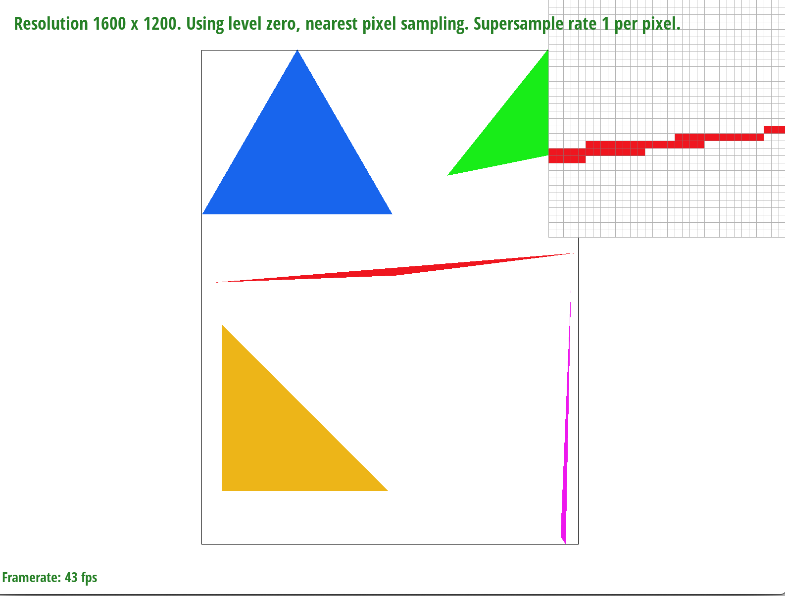
I rasterized triangles by implementing a function called rasterize_triangle that took in three vertices and a color as parameters. Given these vertices, I computed a bounding box for the triangle and iterated through each pixel in this box. For each pixel, I then check that it passes my is_Inside helper function, which when called thrice, ensures that the sample (center point of the pixel) is within a triangle. Additionally, I added support for both the clockwise and counterclockwise directions. If the sample is contained within a given triangle, I pass it as an argument to the fill_pixel function, which adds the given color's rgb values to their appropriate indices in the framebuffer.

Part 2: Antialiasing triangles

To implement supersampling, I updated the rasterize_triangle function to iterate through the sample rate number of subpixels of each pixel. I then performed the isInside triangle check in the same way as Task 1. If a subpixel was found to be inside the given triangle, I would call fill_supersample, a helper function that calculates the correct index of the supersample_buffer and adds a given color as the value at that index. The supersample buffer was a data structure that was sample rate times larger than the framebuffer, and allowed supersampling support because it accounted for subpixel values. I also modified the fill_pixel function to add the original points and lines from the SVG file into the supersample_buffer. Once the supersample_buffer was correctly filled with subpixel sample values, I averaged the subpixel color values for each pixel and added the averages to the framebuffer in the resolve_to_framebuffer function. An important part of supersampling also consisted of managing the memory of the supersample buffer. To handle this, I resized the supersample buffer in set_sample_rate, set_framebuffer_target, and clear_buffers. Supersampling is useful because since we are sampling more times, the resulting image quality is higher. By having a higher sampling rate and then taking intermediate values by averaging, we can use supersampling to antialias our triangles. Having intermediate values will result in softer edges, a more finely rendered image, and fewer artifacts such as jaggies. Overall, the supersampling algorithm maintained the logic of the original rasterization pipeline. However, instead of directly adding to the framebuffer, supersampling called for an intermediatary supersample buffer that could temporarily store all of the subpixel values before averaging them to put into the framebuffer. Also, the isInside triangle checks were applied to each subpixel sample, rather than each pixel.

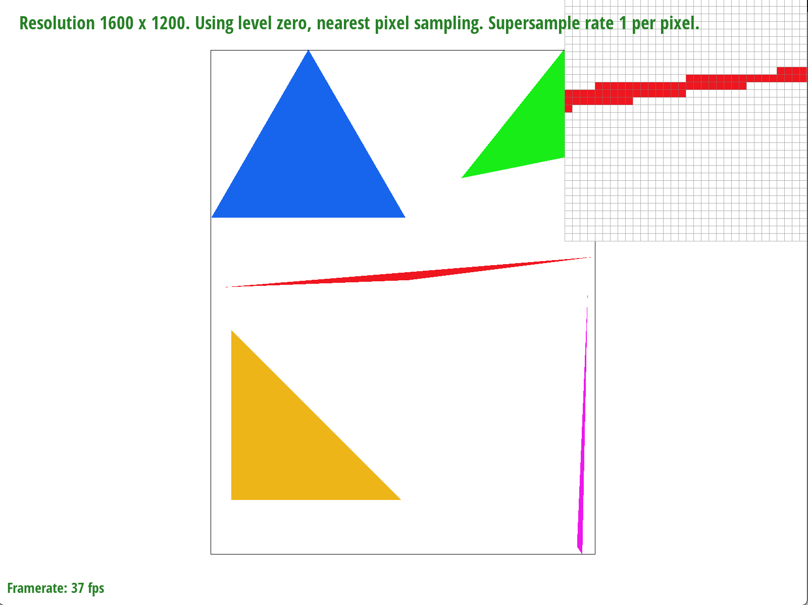
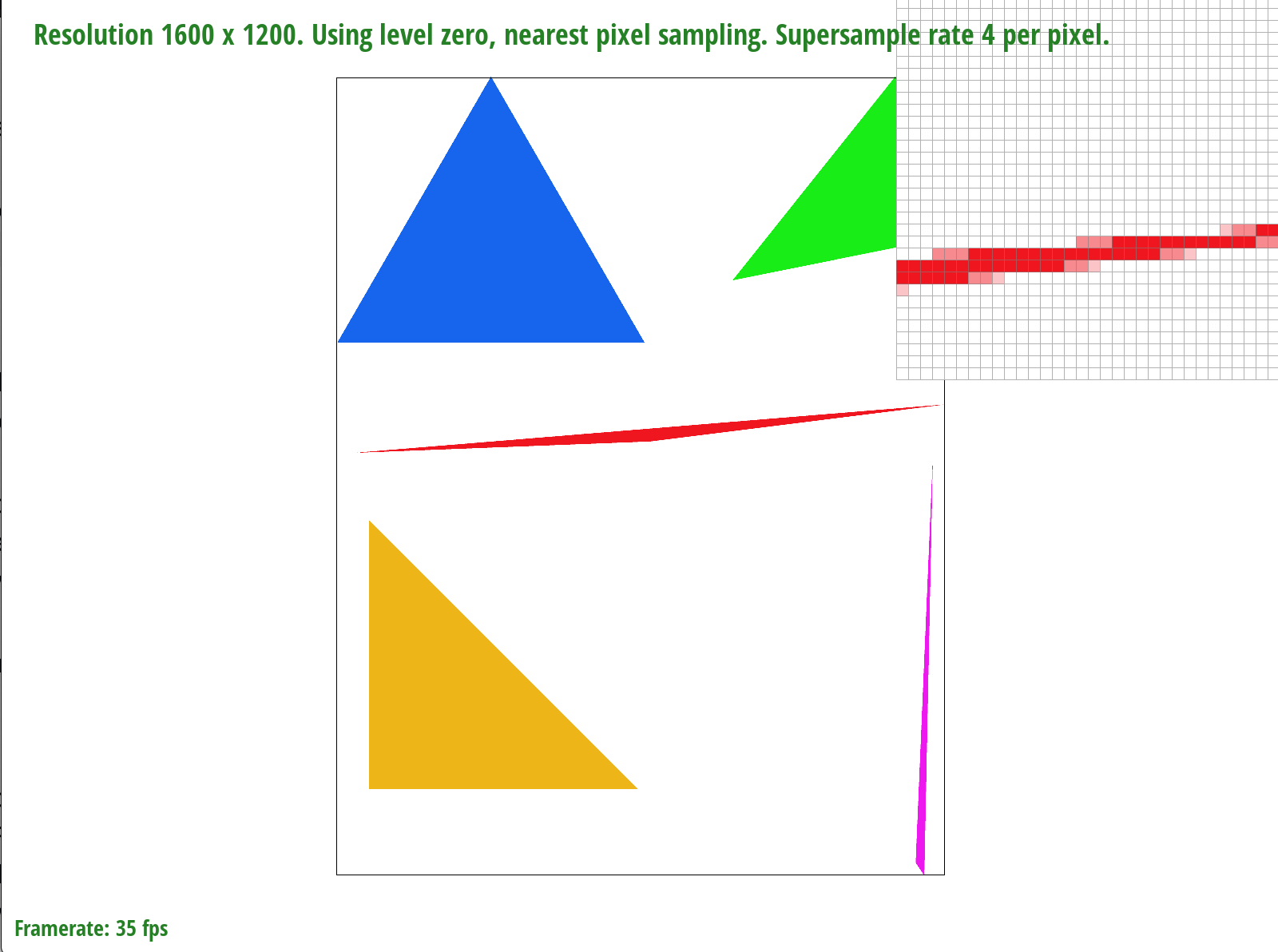
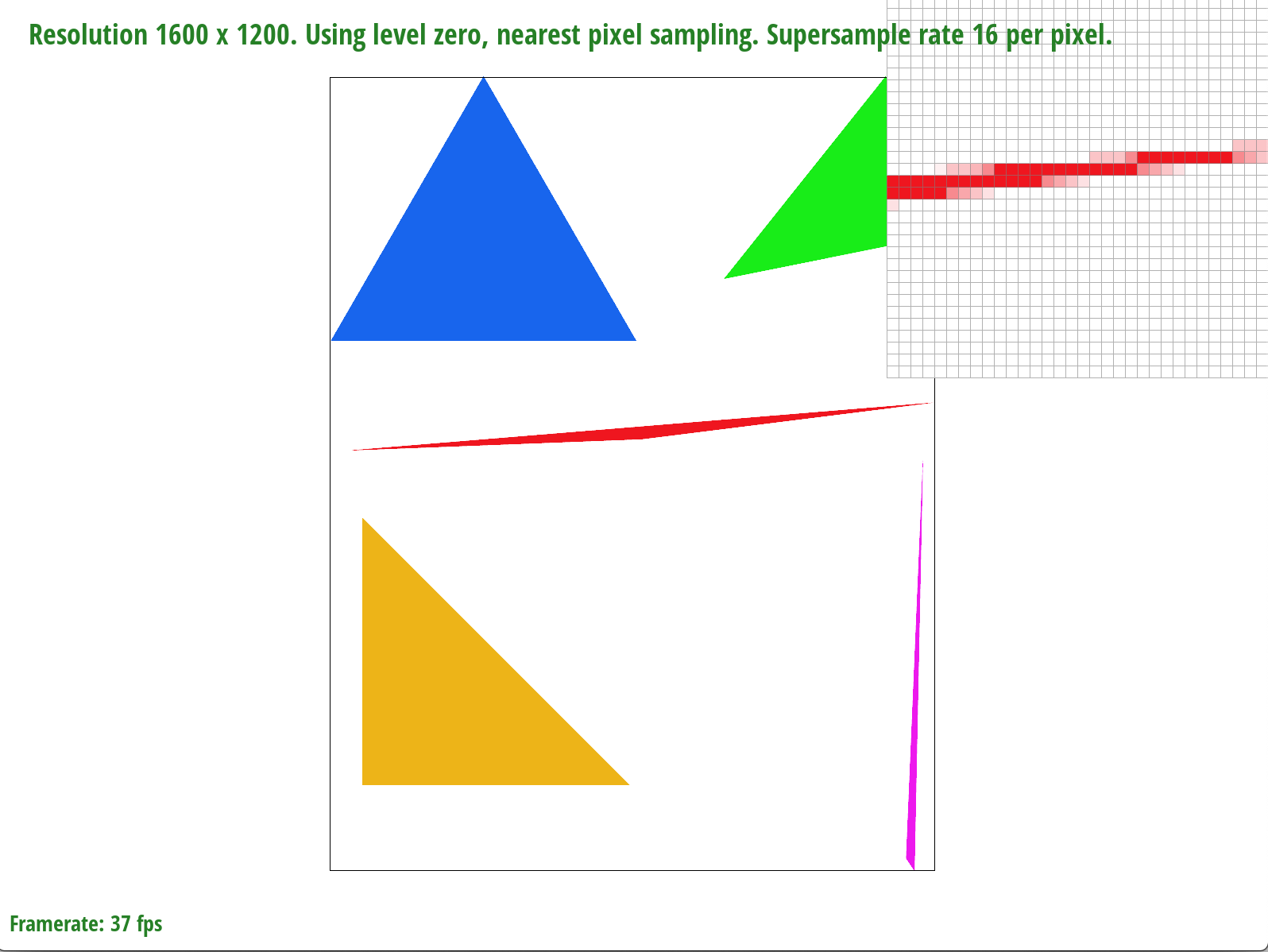
As the above images show, an increase in sample rate results in blurrier edges of the triangle. We are adding precision by sampling more values per pixel, and a result of averaging these values, we are left with a gradient of color rather than jagged edges.

Part 3: Transforms

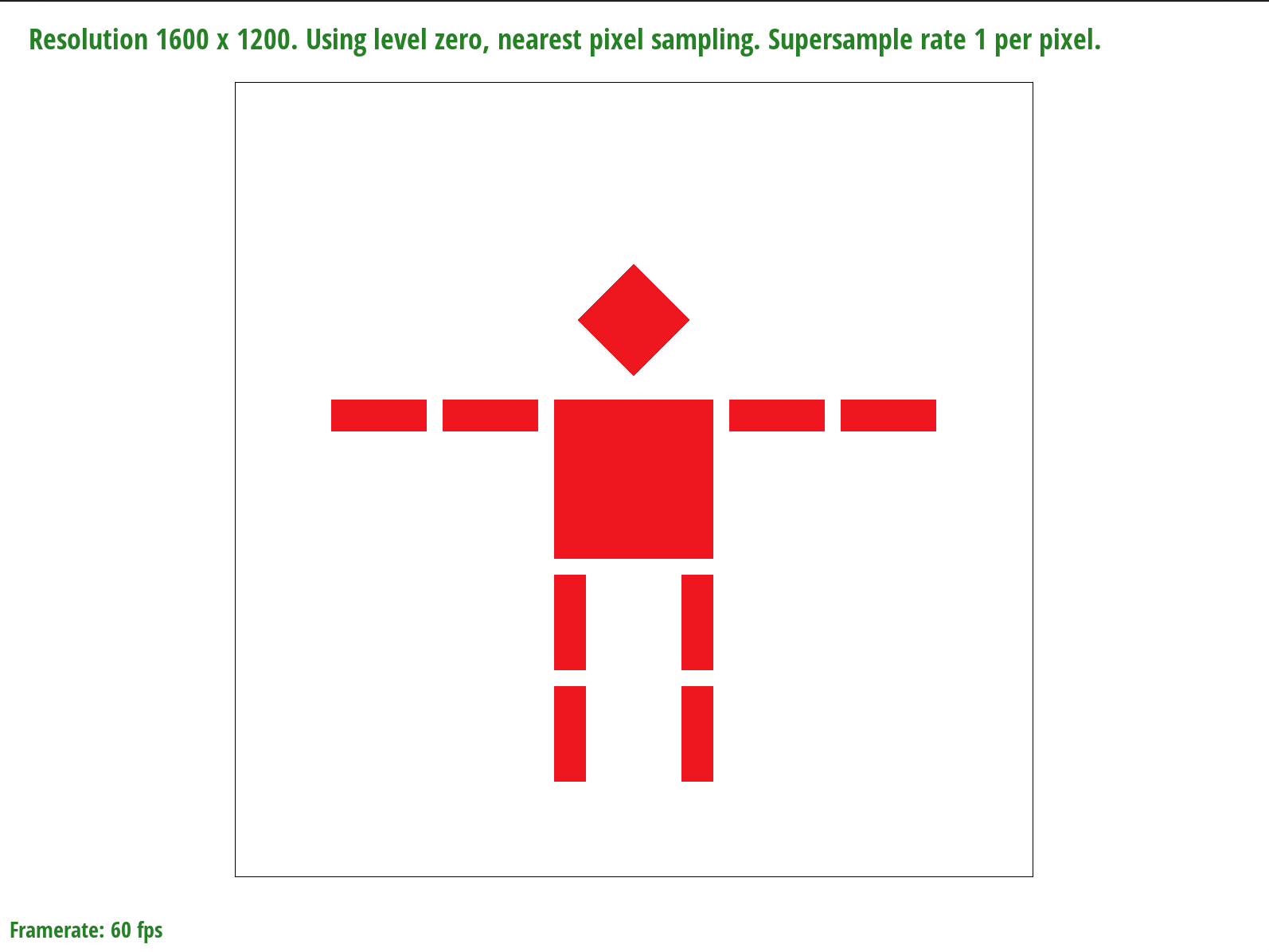
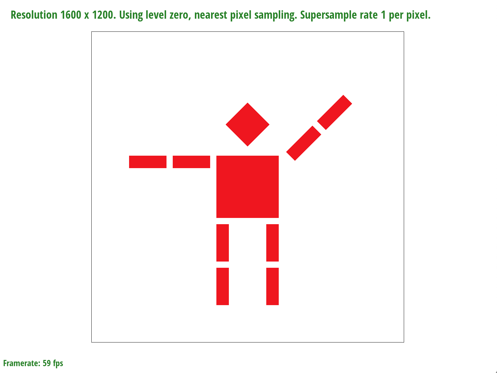
I made the cubeman wave by translating the right arm up by 30 degrees and rotating it counterclockwise by 45 degrees.

Section II: Sampling

Part 4: Barycentric coordinates

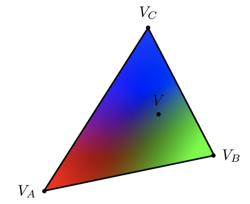
Barycentric coordinates are weights that we can use to represent a point by computing a weighted average of triangle vertices through the following formula:

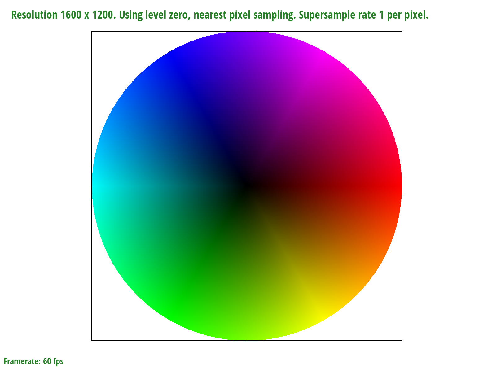
We can use Barycentric coordinates to represent colors – for example, in the image below, each vertex of the triangle represents one color: red, orange, or black. By interpolating the values at the triangle vertices, we can compute the color of each pixel and form a gradient over the triangle. To exemplify this concept, we can see that the pixel coordinates closer to the black vertex are darker than those closer to the red vertex. Likewise, the pixels closer to the red vertex are more red; therefore, the weight of the vertex in the value of a particular pixel is proportional to its distance to the pixel.

Part 5: "Pixel sampling" for texture mapping

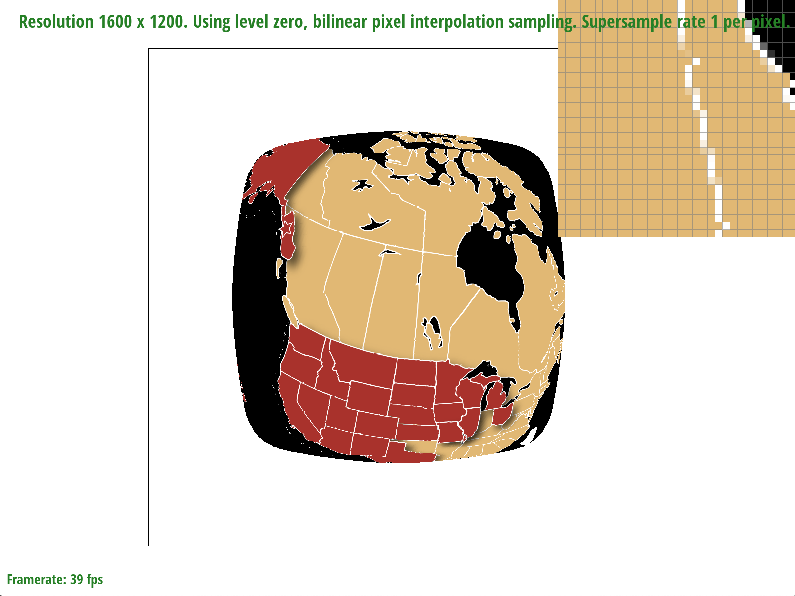
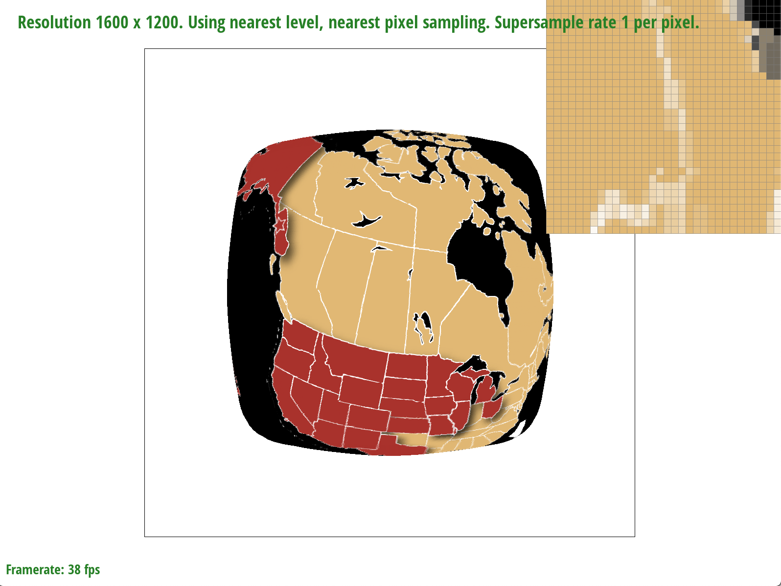
Pixel sampling is the process of mapping from the screen space to the texture space and sampling texels from the texture space. I implemented pixel sampling by comverting (x, y) screen sample coordinates to (u, v) coordinates and scaling those by the texture width and height to get tx, ty coordinates, or texture samples. Nearest pixel sampling sets the color of a pixel to be the texel color associated with the tx, ty coordinates closest to the sample in question. Bilinear sampling sets the color of a pixel by performing linear interpolations on the four surrounding pixel coordinates. More specifically, to implement bilinear sampling in this project, I linearly interpolated across the two top and two bottom coordinates, and then interpolated vertically between them.

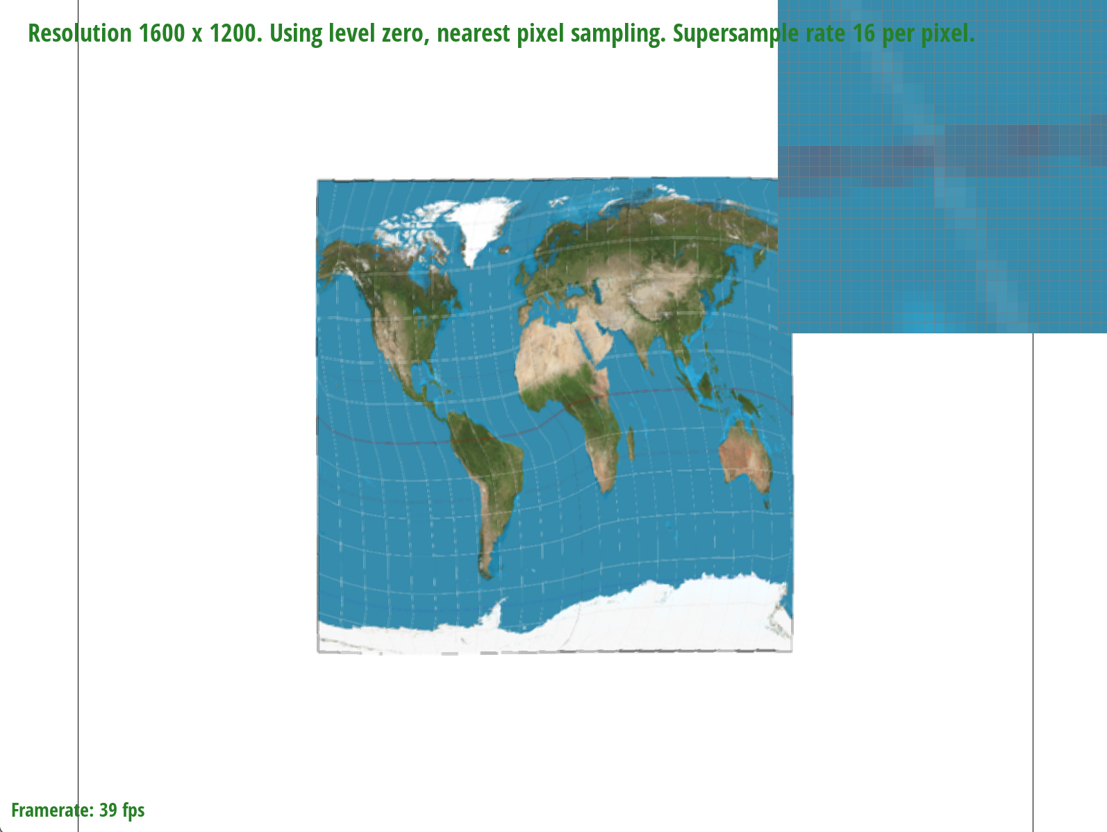
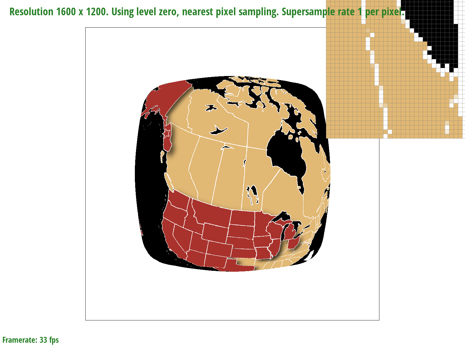
The differences between bilinear sampling and nearest pixel sampling are much more evident at lower sample rates, which makes sense because given fewer samples, the information contained by each sample and the effectiveness of a sampling method to retrieve it becomes magnified. At a sample rate of 1, for example, bilinear sampling is more effective at connecting the latitude and longitude lines on the map by blurring the edges. In the nearest pixel sampling image, on the other hand, we can see a disconnect in the lines, meaning that some information is missing. At a higher sample rate of 16, the differences are less noticeable; however, bilinear sampling seems to produce slightly finer and more precise lines than nearest pixel sampling.

Part 6: "Level sampling" with mipmaps for texture mapping

Level sampling can be used to solve the problem of minification, where we want to downsample such that our pixels include a greater number of texels. In this type of sampling, we sample from different levels of a mipmap, a hierarchical structure where the bottom level stores the highest resolution and the top level stores the lowest. I implemented level sampling by finding p_dx_uv and p_dy_uv, which involved computing the barycentric coordinates for every subpixel (xi, yi), as well as those for (xi + 1, yi) and (xi, yi + 1). I then passed these vectors into my helper function get_level, which scaled the uv coordinates by the texel width and height, and returned my desired mipmap level.

Supersampling is a method that effectively implements antialiasing, however its high-quality results come with the tradeoff that it is costly to compute information for so many samples. Nearest pixel sampling, on the other hand, is faster and less complex in terms of computational power; however, it results lower quality images. In terms of computational cost, bilinear sampling is slower than nearest pixel sampling because it requires calculations involving the four nearest samples to a point, but it is faster than supersampling because we are still checking fewer samples. Overall, supersampling and bilinear sampling will produce higher quality images at different zoom levels, but supersampling is slow and uses the most memory (necessitates the creation of a new supersample buffer). Level sampling scales the quality of an image depending on the mipmap level used. For example, the lowest level (0) will produce the highest quality image because it stores the most information in memory, thus making it also the most costly to compute. Higher levels in the mipmap pyramid will require less memory but will as a result also store less information.

MeshEdit

Overview

In this project, I implemented de Casteljau's algorithm to build Bezier curves and surfaces. I also implemented loop subdivision, an upsampling algorithm that used edge flipping and splitting over halfedge meshes to increase their resolution. I thought it was interesting how pre-splitting edges could alleviate asymmetry when performing loop subdivision, because it could fix the uneven distribution of triangles.

Section I: Bezier Curves and Surfaces

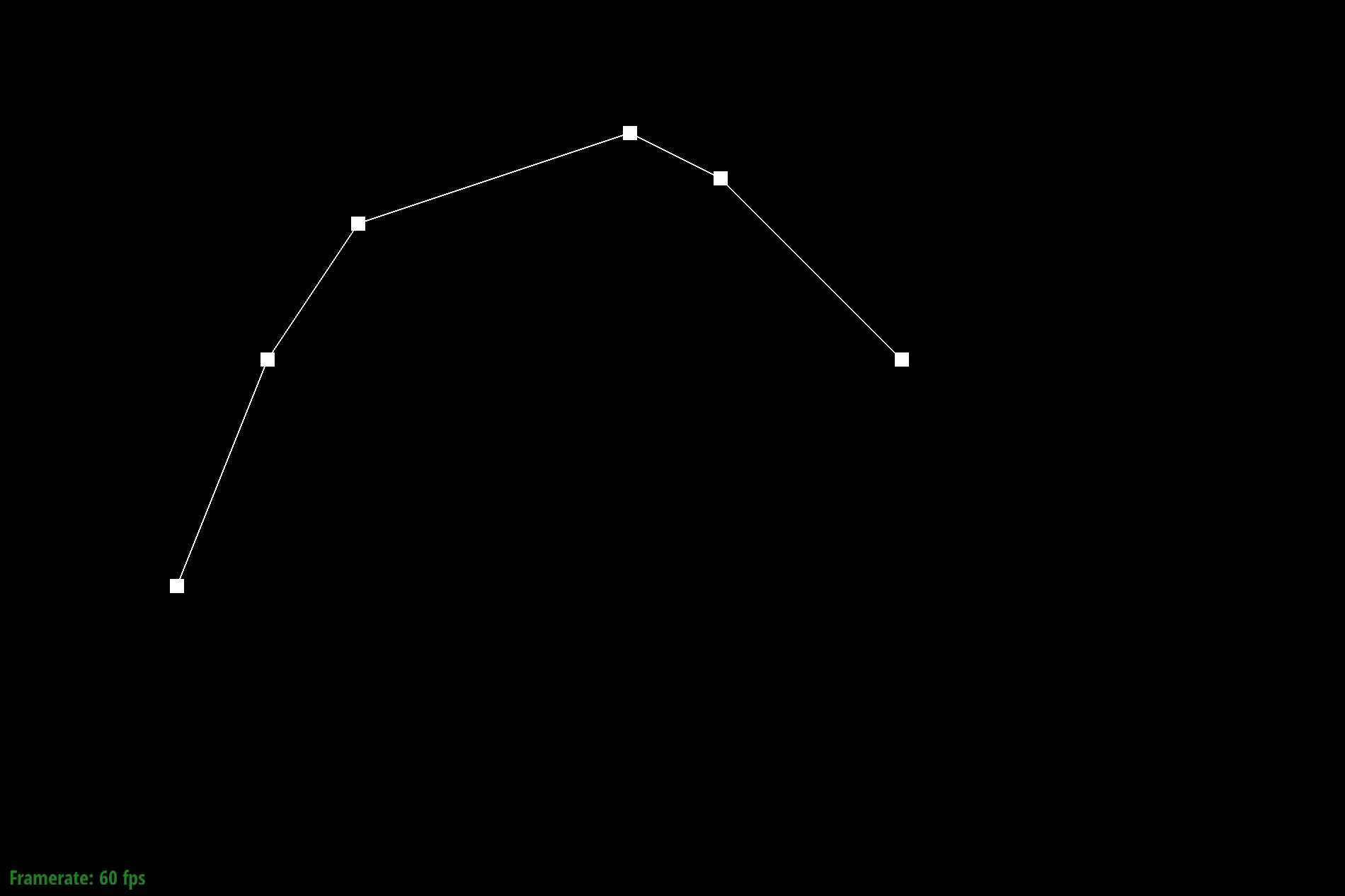
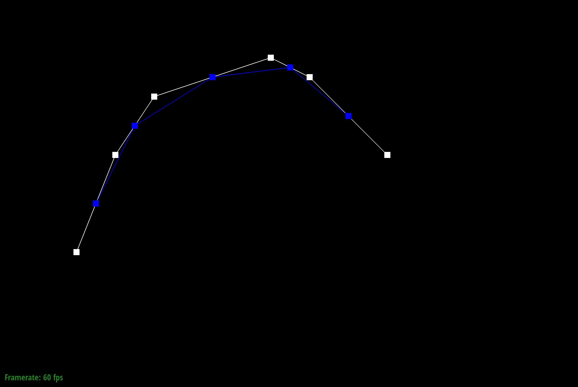
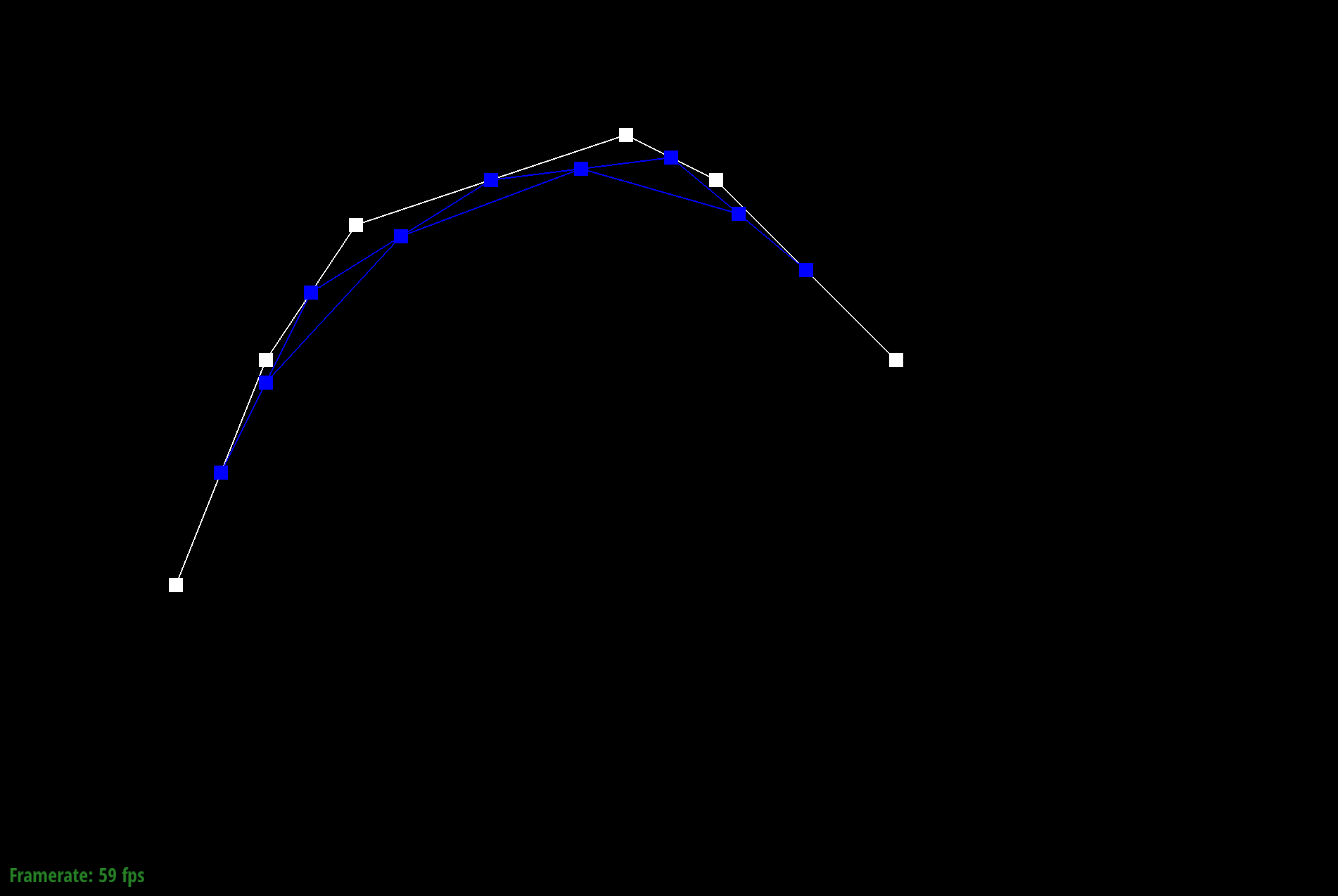
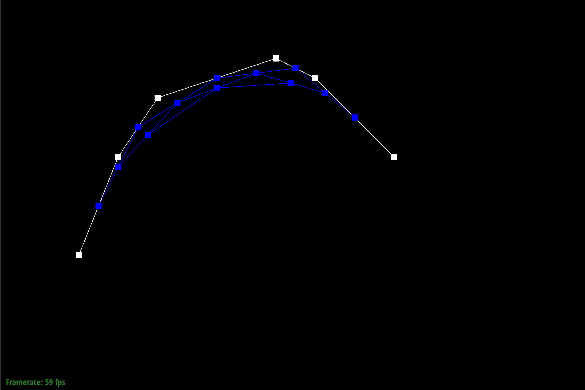
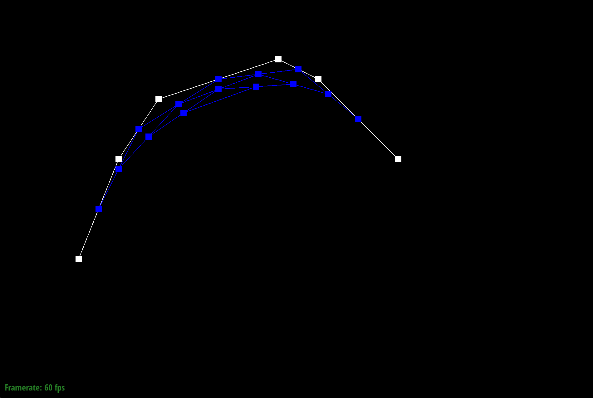
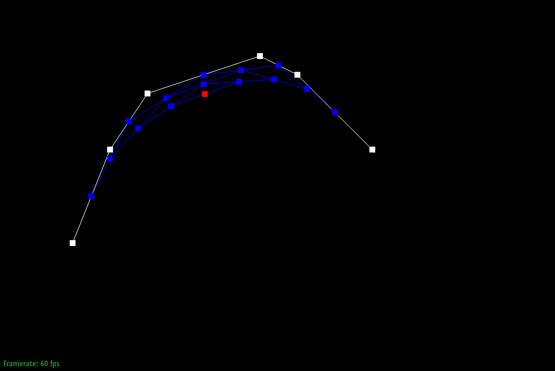
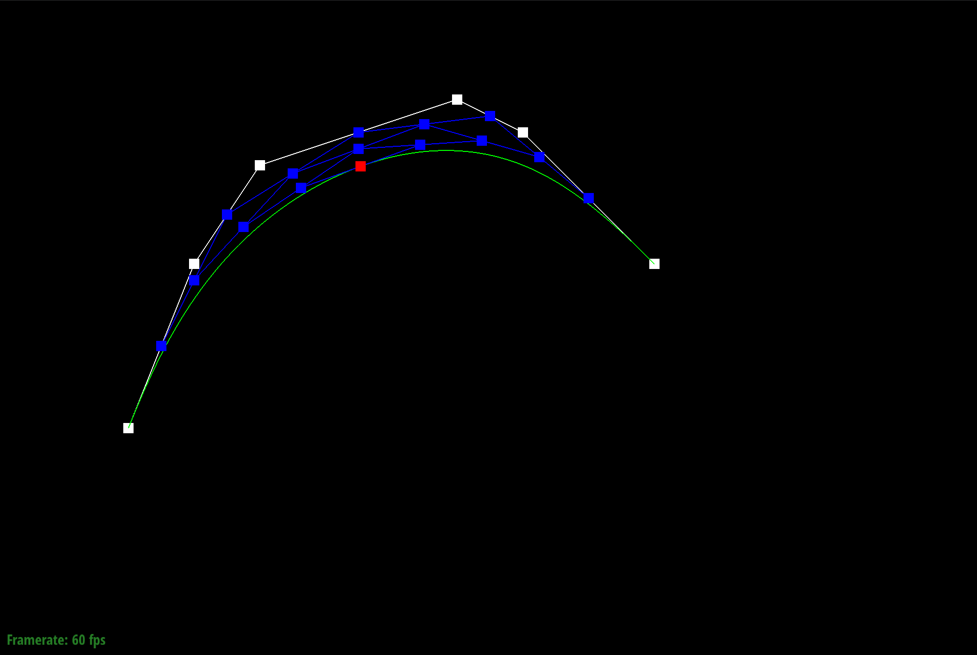
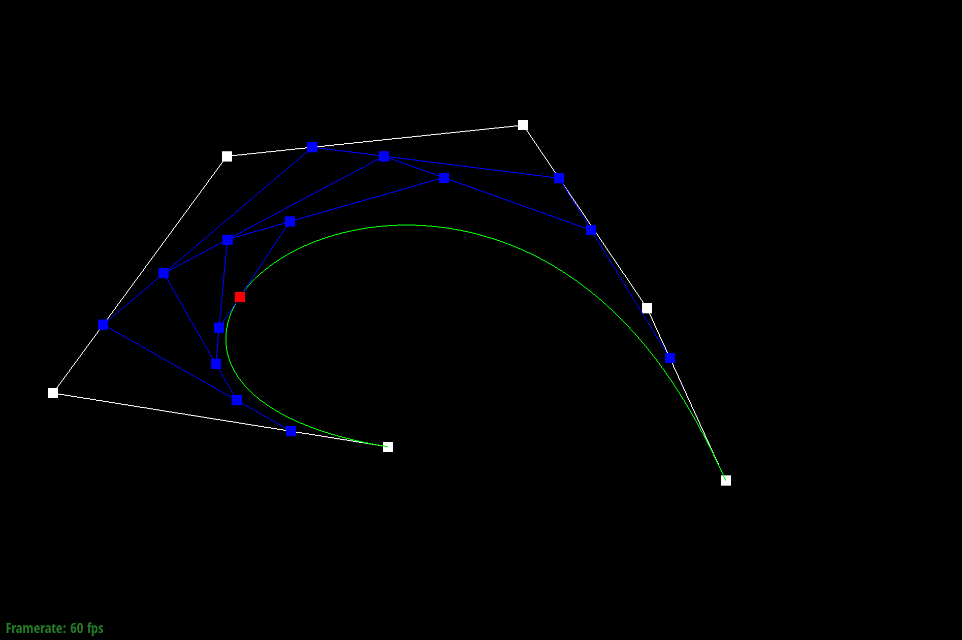
The de Casteljau's algorithm is a recursive solution to evaluating Bezier curves by performing successive linear interpolation across a given number of points. So given n control points, I implemented one step of this algorithm by linearly interpolating to compute the n-1 derivatives, or intermediate control points. By continually calling this evaluateStep function, I am able to successively interpolate until I have one point that represents a final point on my curve. The parameter t takes on values between 0 and 1, and changing this parameter results in the computation of different points of the final curve. So by sliding the values of parameter t, we can perform de Casteljau's algorithm to compute the full curve.

Part 1: Bezier curves with 1D de Casteljau subdivision

Part 2: Bezier surfaces with separable 1D de Casteljau subdivision

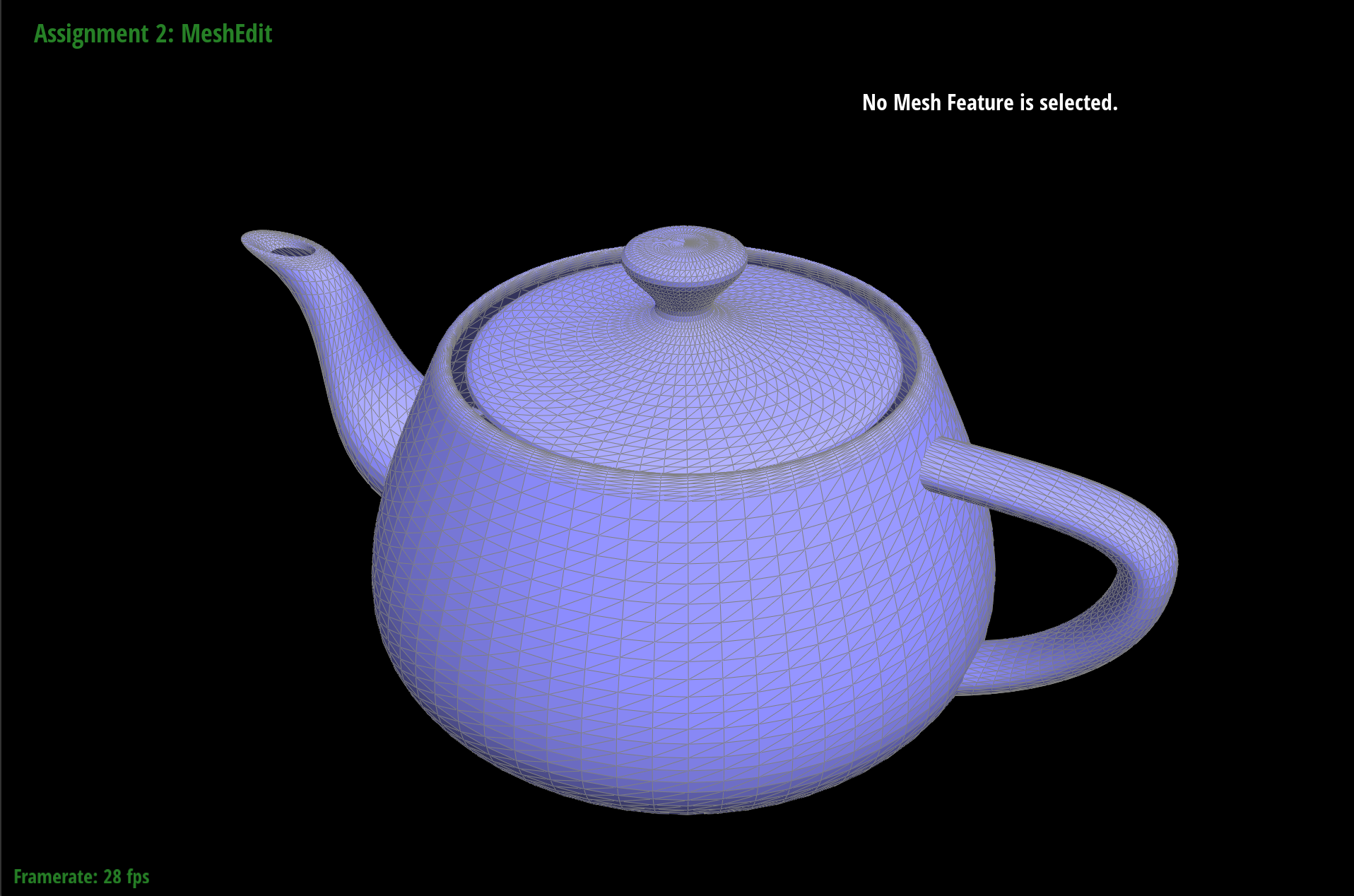
A Bezier surface is comprised of m rows of control points, where each row forms a Bezier curve parameterized by u. The cross-section of these m rows then form n rows of control points. As a result, we can see a Bezier surface as a sort of matrix, and perform de Casteljau's algorithm successively to the m rows and then n columns. In my implementation, I divided this task into an evaluate function, coupled with two helper functions. The first helper function, evaluateStep, had the same utility as evaluateStep in Task 1, only it accounted for the 3-D space instead of just the 2-D. The second helper function evaluate1D successfully calls evaluateStep to return one final point on a Bezier curve. The final function evaluate calls evaluate1D to compute a P_i parameterized by u for m rows in my "matrix" of control points. I then allocate space for a vector that stores these P_i points, and call evaluate1D once more to evaluate these P_i points in the column direction, to return one final point on the Bezier curve parameterized by both u and v.

Section II: Sampling

Part 3: Average normals for half-edge meshes

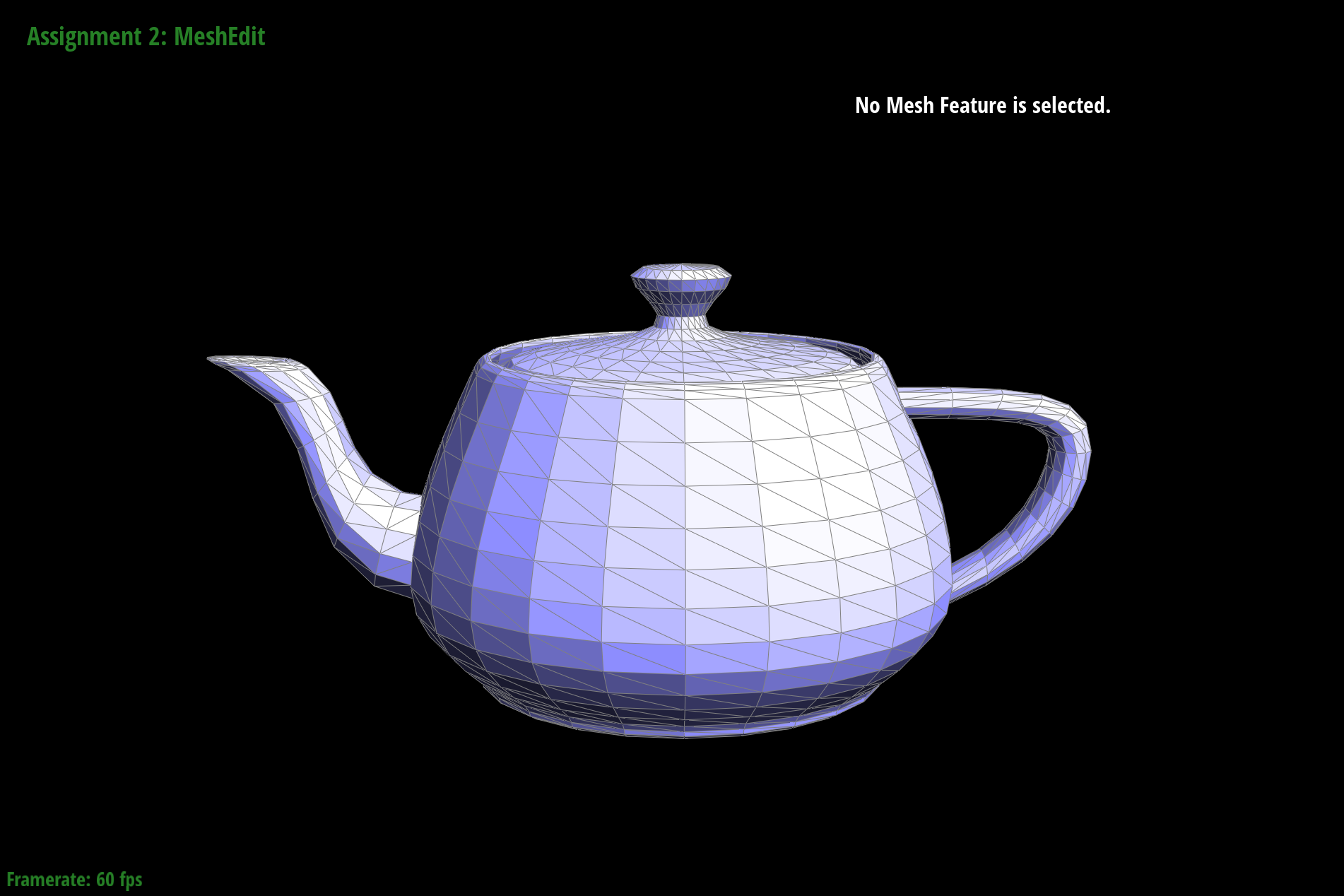
I implemented the area-weighted vertex normals in the function normal, where given a vertex, I iterated through all of the neighboring vertices to compute the area of each face using the cross function. I summed up the areas and then divided by the number of faces to compute an average, then I called unit on this result to normalize it.

Part 4: Half-edge Flip

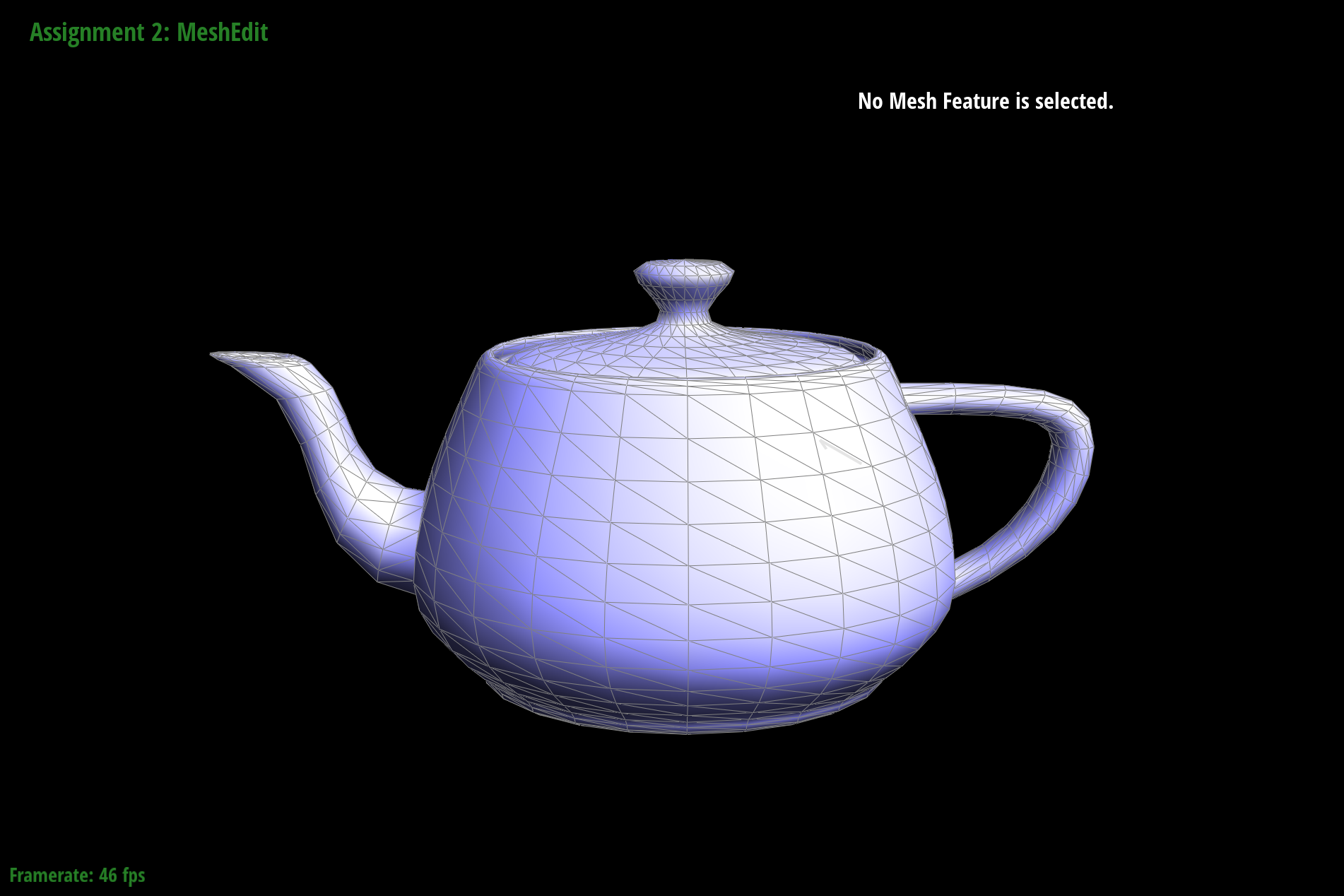
My implementation of the edge flip operation consisted of initializing the values for a mesh and flipping a given edge, which entailed reassigning values and pointers to all relevant mesh elements. To write the flipEdge function, I relied on the "Guide to Implementing Edge Operations" document. By following the provided reference document carefully, I was able to avoid any major debugging.

Part 5: Half-edge Split

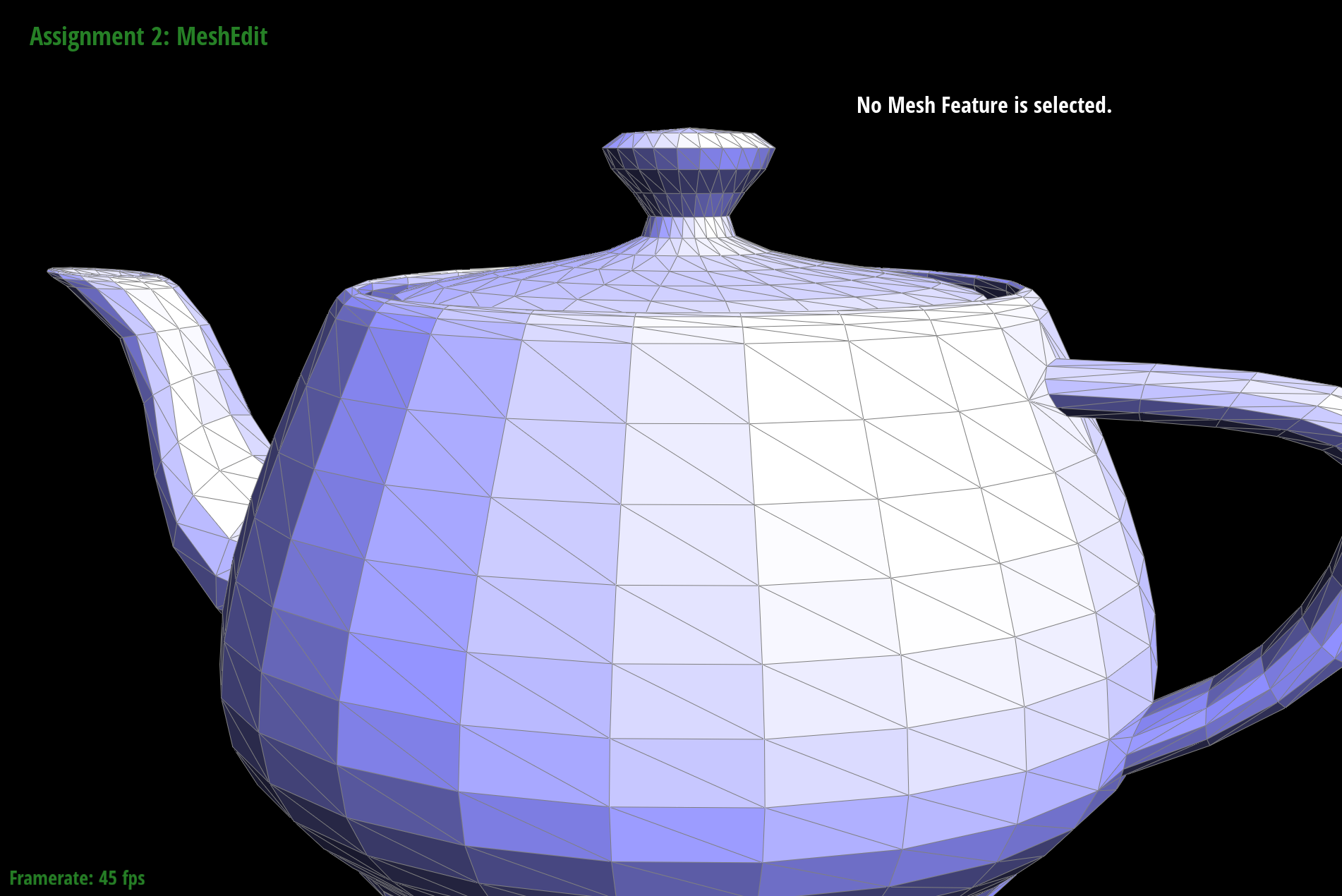
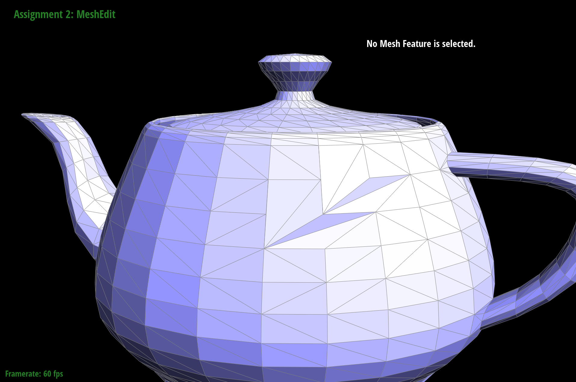
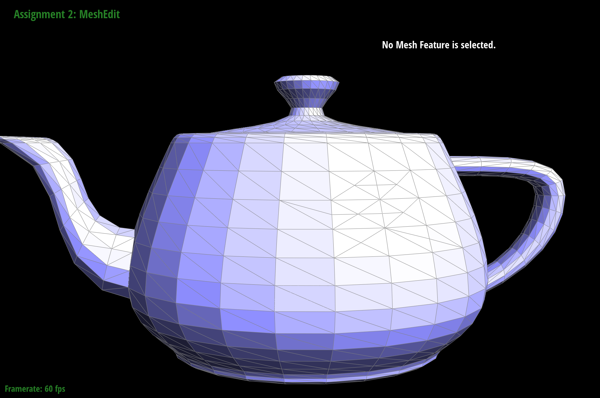
To implement the edge split operation, I followed the same process for initializing my mesh as in Task 4. However, edge splitting was more complicated than flipping because I had to create new mesh elements to support the split operation, as well as compute the position for the new vertex, which was the midpoint of the vertices that were on either side of the given EdgeIter e0. I then drew my own after-split diagram to figure out how to reassign element pointers, and followed the diagram in my code implementation. I debugged this section by repeatedly checking that my diagram matched with my actual implementation. While I was able to fix some pointer errors this way, ultimately I realized I was creating my new elements incorrectly. Originally I was creating a new object for each element (e.g. calling EdgeIter() to create a new EdgeIter), whereas I should have been calling the new______ function (e.g. newEdgeIter()).

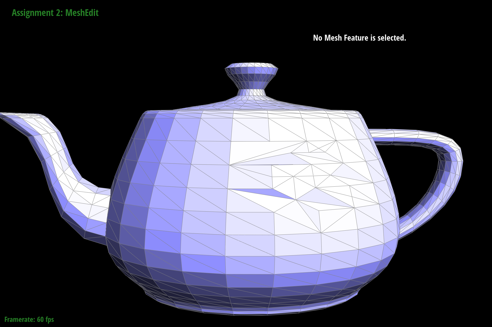
Part 6: Loop subdivision for mesh upsampling

I implemented loop subdivision in three steps. In the first step, I iterated through the old vertices and pre-computed their positions – that is, I calculated what their values would be after splitting and flipping edges. I also pre-computed the positions of the new vertices that would be created from edge splitting, and stored their positions in the newPosition member variable of the Edge class. In the second step, I call splitEdge and flipEdge, making sure to only split edges that existed in the original coarse mesh and flip new edges that connected an old vertex and a new vertex. To keep track of new edges and vertices, I altered my implementation of Task 5 by setting the property isNew to true for the new vertex and new edges created. In the final step, I update the old vertex positions to their new positions in the upsampled mesh, and set the positions of the new vertices using the precompute values from the first step.

As we can see from the following screenshots, meshes become smoother after loop subdivision, and sharp corners and edges become rounded.

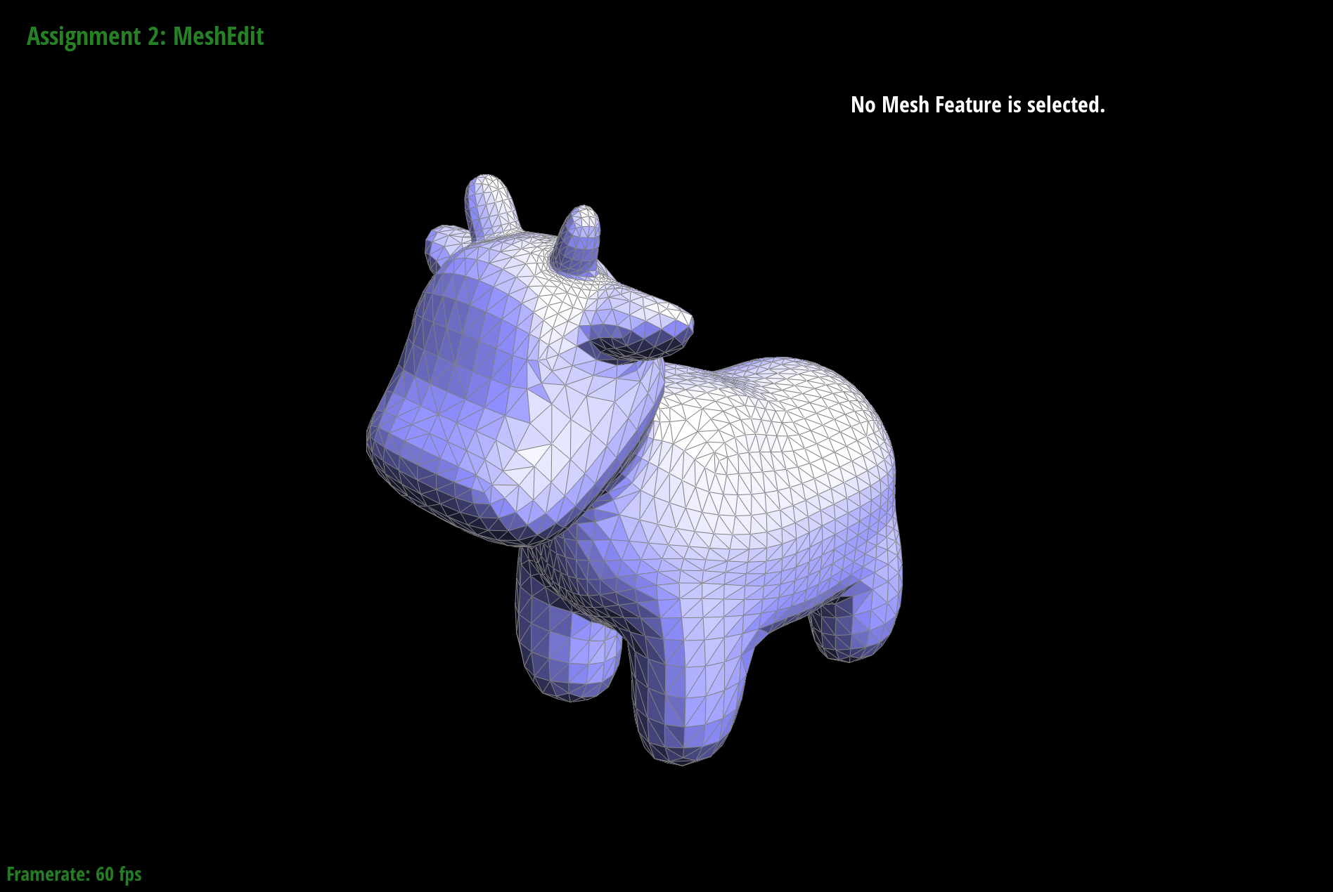
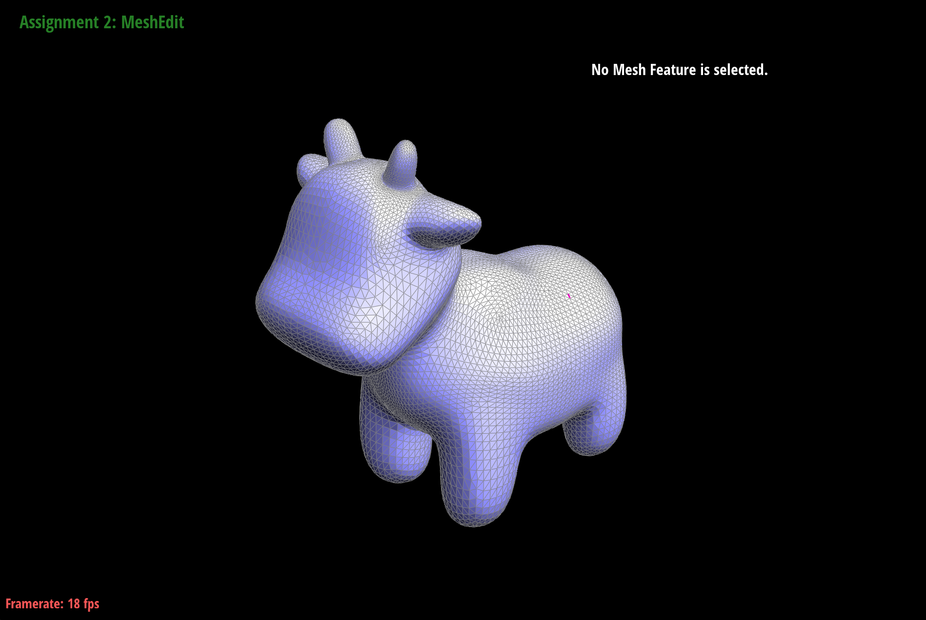
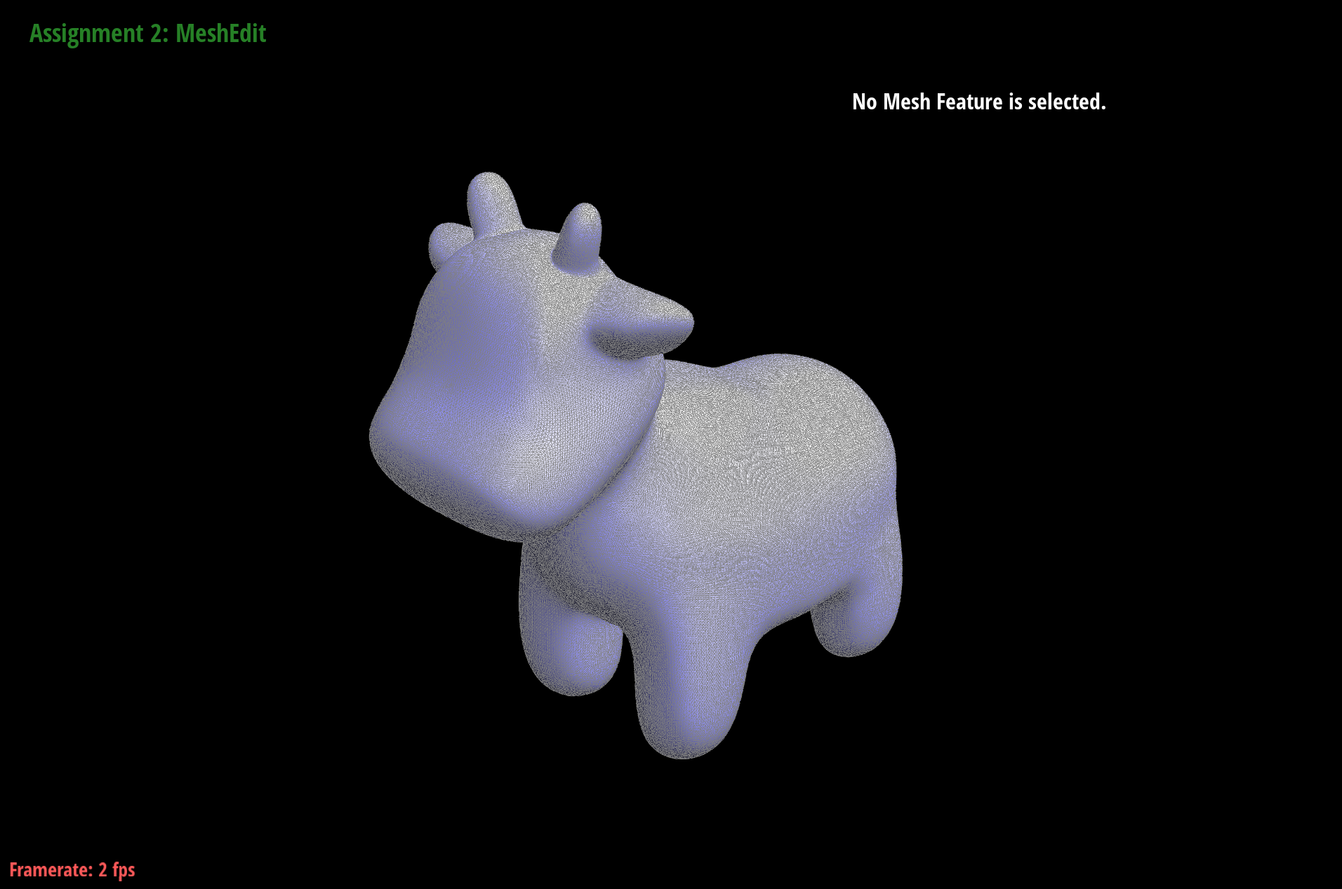
We can reduce this rounded effect by pre-splitting edges along the sharp corners – this process works because having more edges means that we're sampling more points and preserving the original mesh shape. The presplitting process is demonstrated on a cube in the below screenshots.

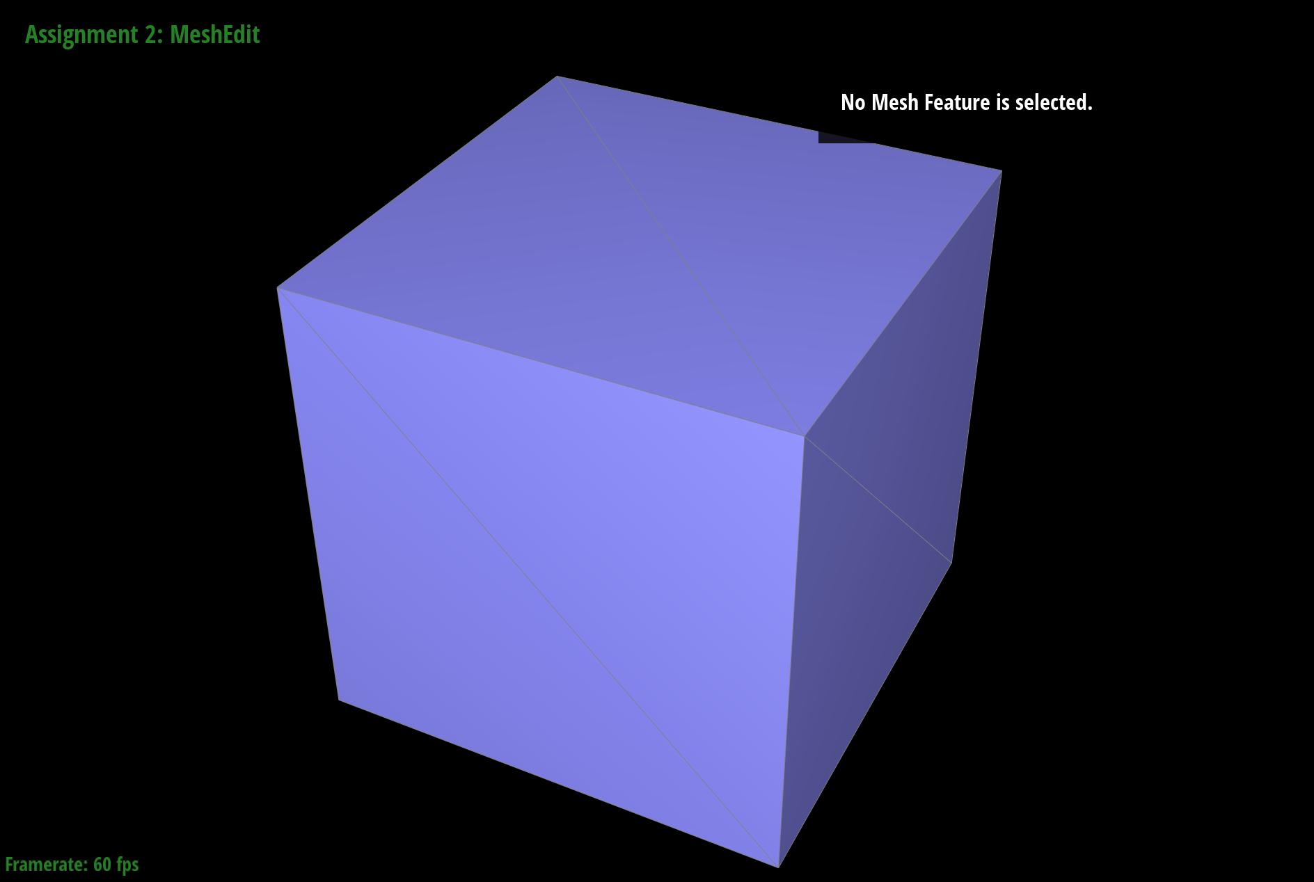
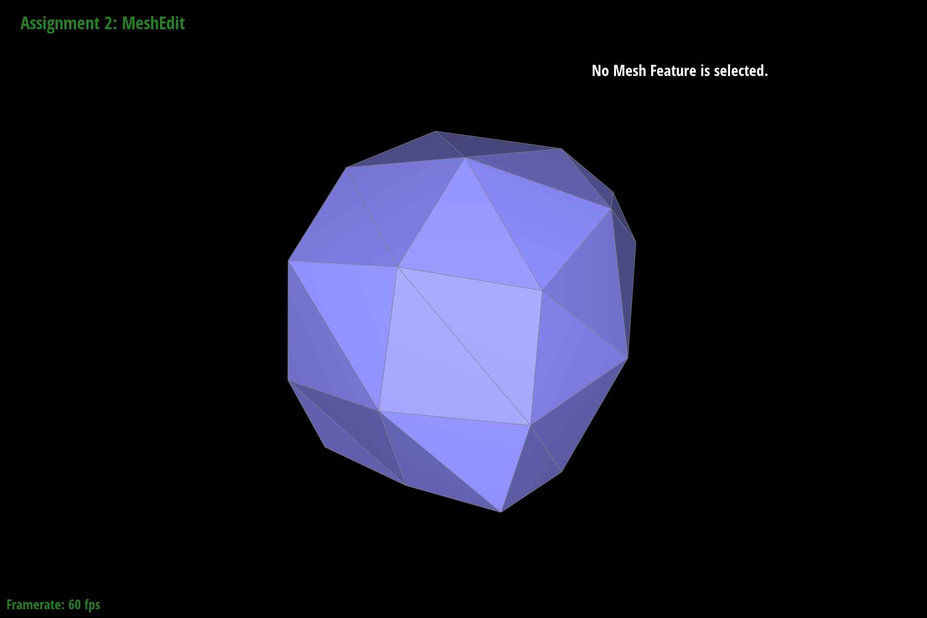
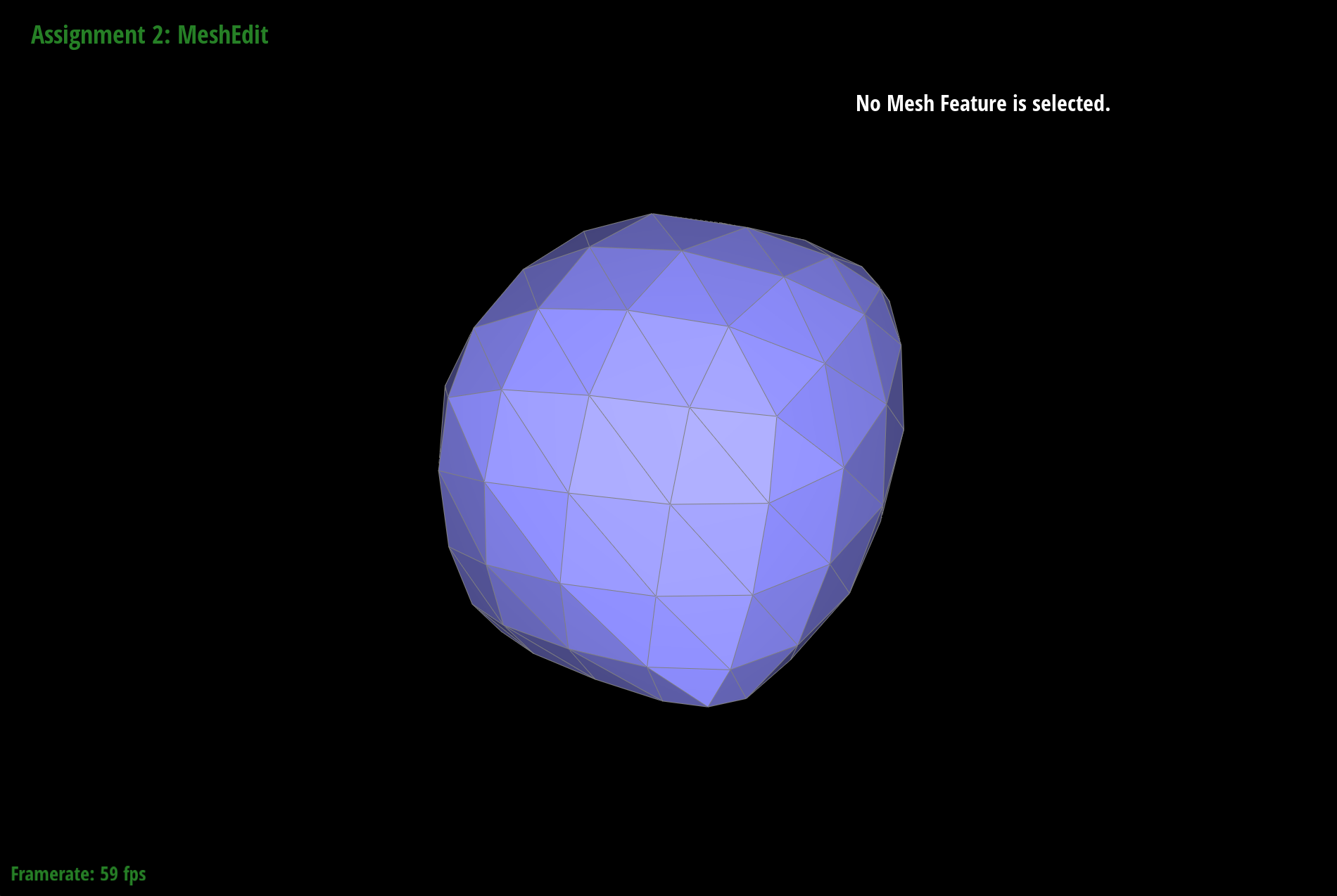
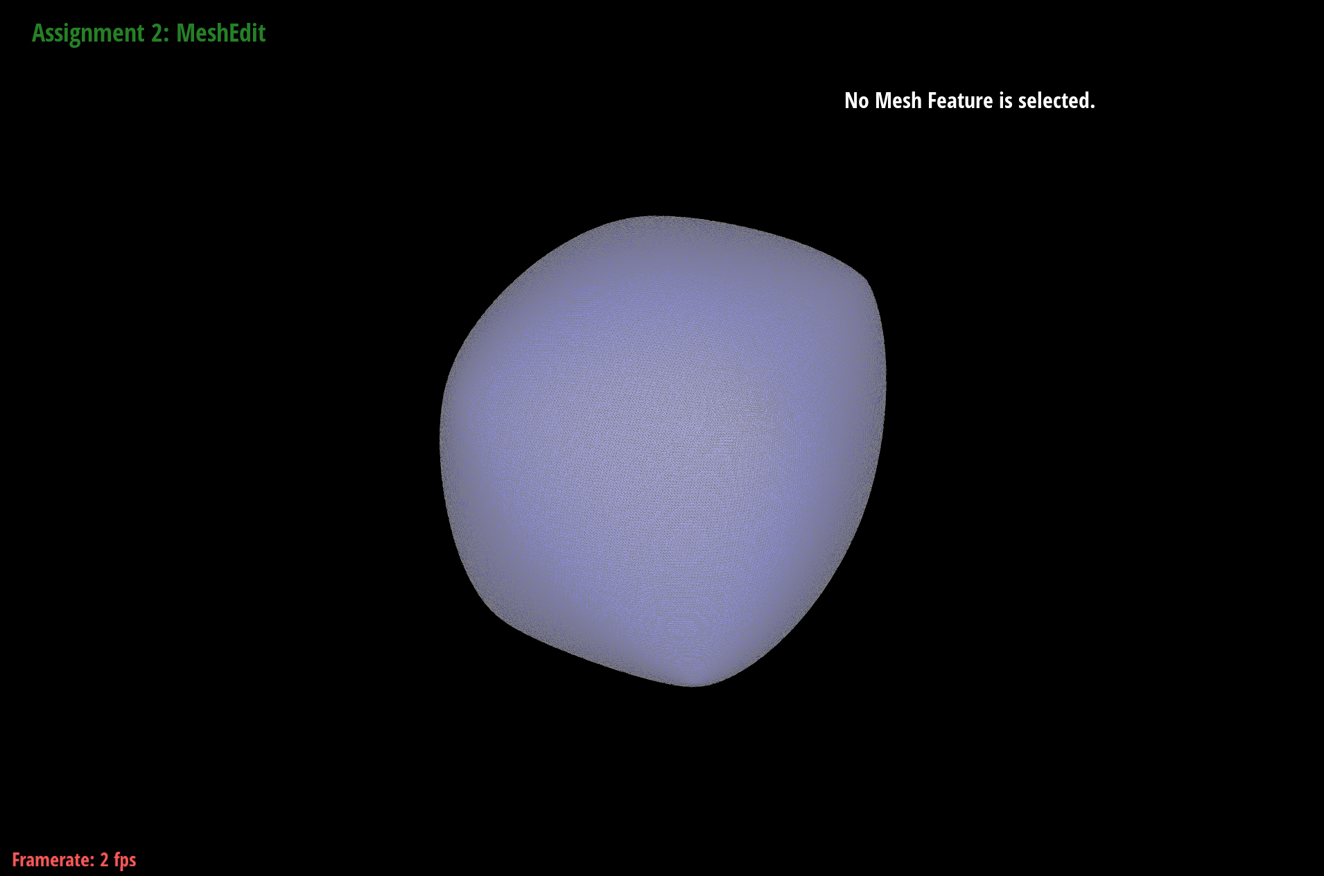
The cube becomes more symmetric after repeated subdivisions; is seems as if in the images, certain corners (such as the bottom-most) produce less rounding than others. It seems as if this is happening because the triangle meshes that make up the sides of the cube are asymmetrically distributed. Therefore, if we pre-split the edges such that each face is composed of four triangles, we are left with a more symmetrical distribution such that each face subdivides in the same way every time we upsample. Below are screenshots of this process:

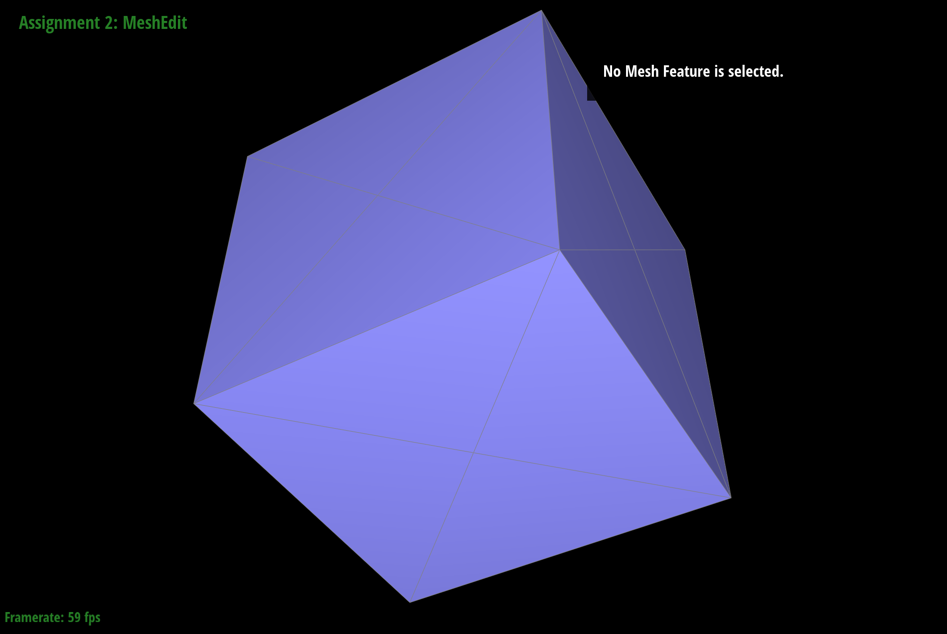
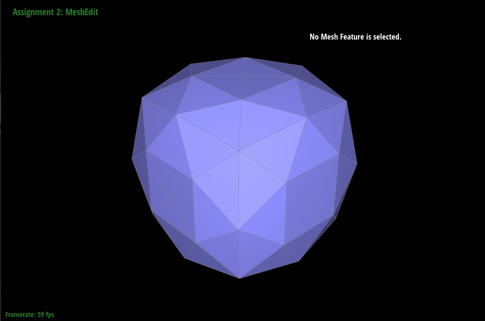
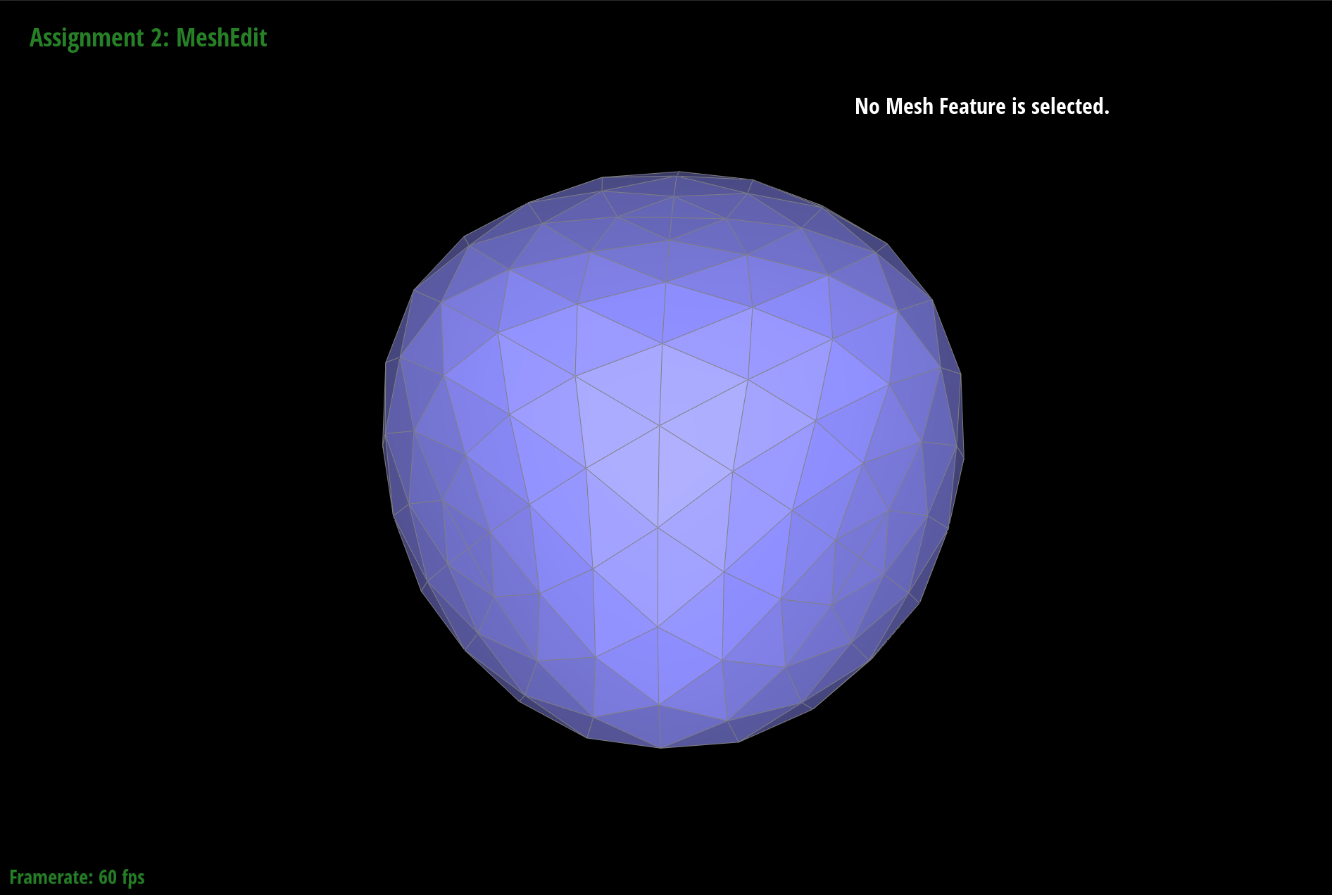
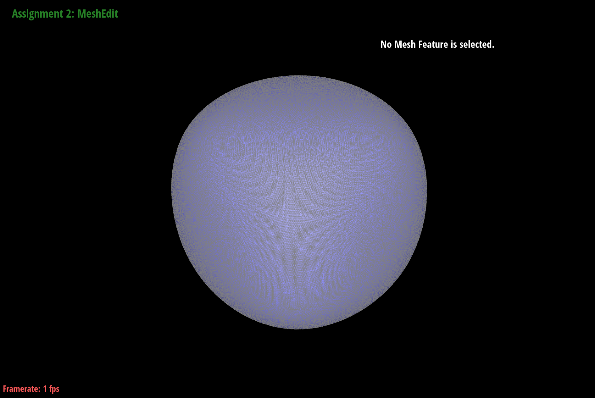
As we can see, pre-splitting alleviates asymmetry.

PathTracer

Overview

In this project, I used a pathtracing algorithm to implement a physically-based renderer. I also added support for complex materials such as mirror and glass and depth of field effects using a thin-lens camera model.

Part 1: Ray Generation and Intersection

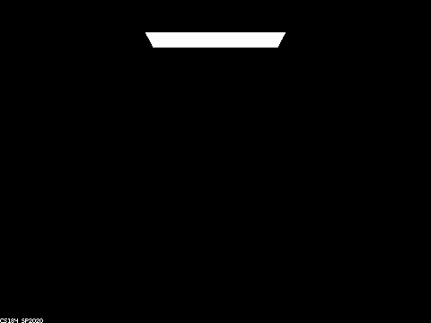
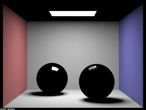
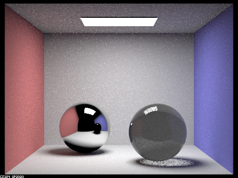
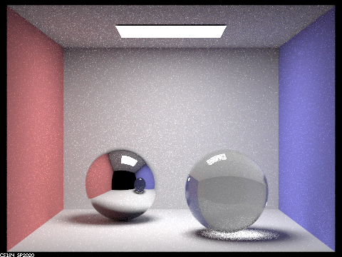
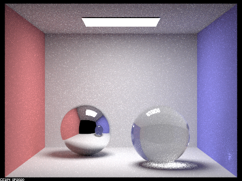
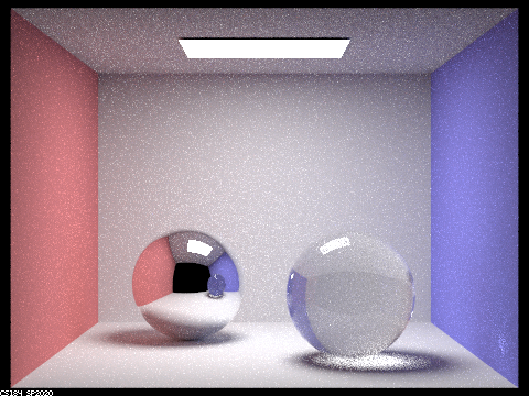
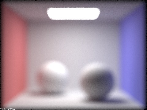
When max ray depth = 0, the scene is black because there are no light bounces, and the only light we receive is that from the source. When max ray depth = 1, we see the results of a one light bounce from the source off onto the surface of the spheres. When max ray depth = 2, the mirror ball looks reflective as the light from the source begins to bounce off of the walls. While the glass sphere has begun to lighten, its reflection in the mirror sphere is still black. It is also only until max ray depth = 3 that we can fully see the transparency of the glass sphere, since it takes more bounces for light to travel through a material. The underside of the glass sphere also becomes much brighter and there is some light reflected onto the wall. When max ray depth = 5, the glass ball becomes a little brighter as more light is bouncing around inside. At max ray depth = 100, the scene is accurately and brightly lit as many rays of light are bouncing off of all of the surfaces.

Part 2: Depth of Field

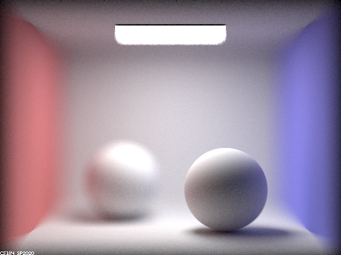
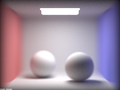
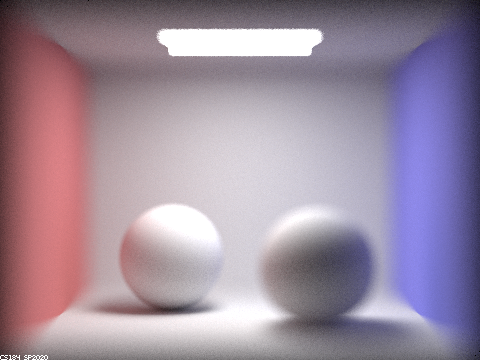
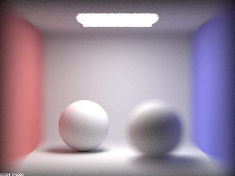
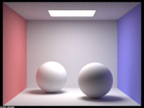
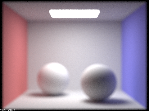
All parts of an image are in focus when we use a pinhole model camera. On the other hand, when we use a thin-lens camera model, different parts of the image are in focus depending on how we choose our lens radius and our focal distance. As a result, the images we get from using a thin-lens camera model are more realistic to how a human eye sees the world than those produced from a pinhole camera.

Cloth Simulator

Overview

In this project, I computed the physics of a mass and spring system to simulate the movement of a cloth. In addition, I added support for collision between the cloth and itself, as well as the cloth and other objects, and I also implemented a variety of shaders.

Section I: Masses and springs

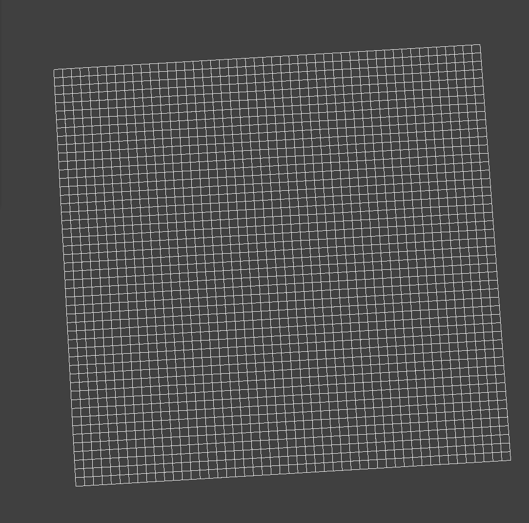
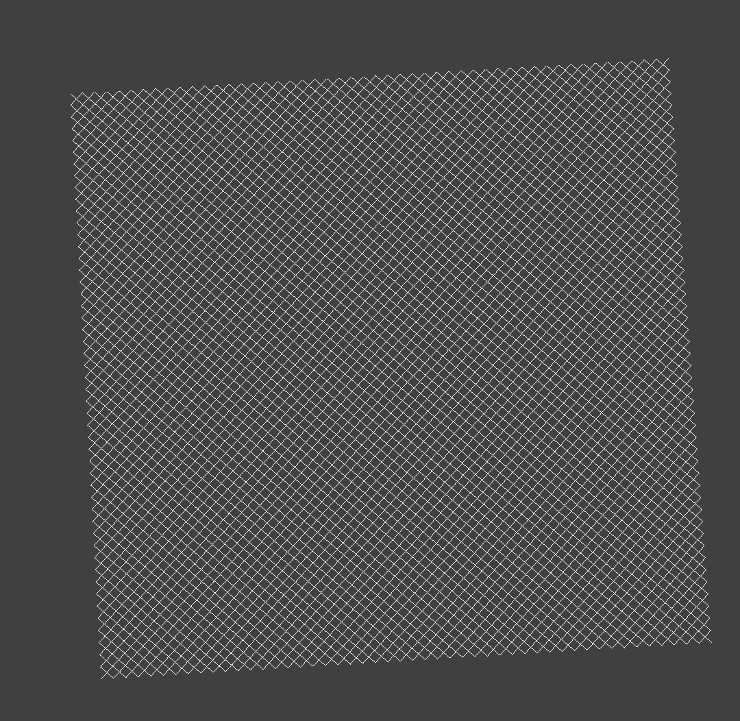
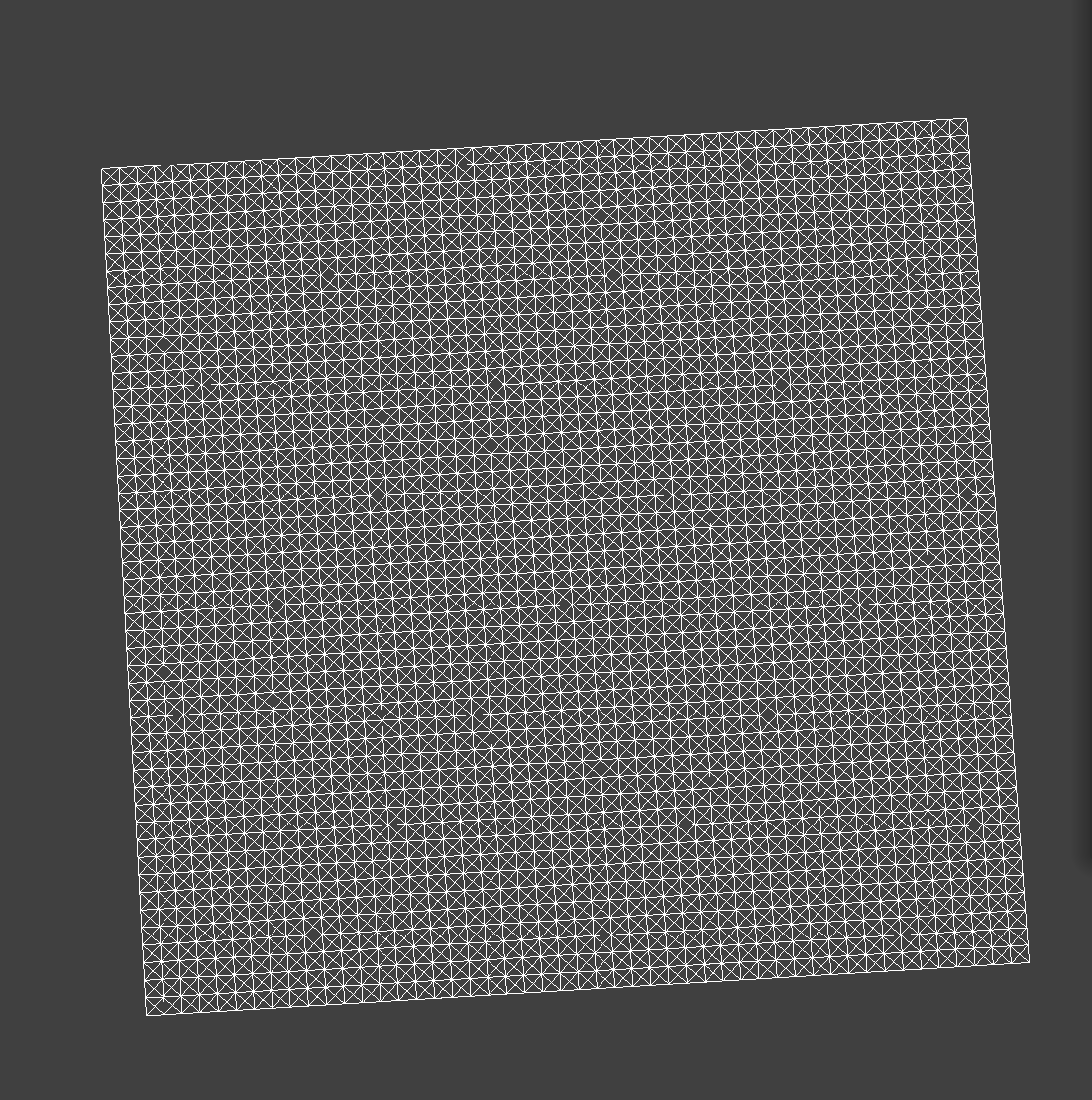
Below are screenshots of a cloth wireframe to demonstrate the effects of structural, shear, and bending constraints.

Section II: Simulation via numerical integration

Changing the spring constant ks controls stiffness. A lower ks will produce a stretchier cloth, whereas a higher ks will produce a stiffer cloth. Compared to the default, for example, the cloth produced with a lower ks value has more wrinkles towards the top, implying a greated flexibility that the cloth produced with a higher ks value, which appears to have fewer wrinkles.

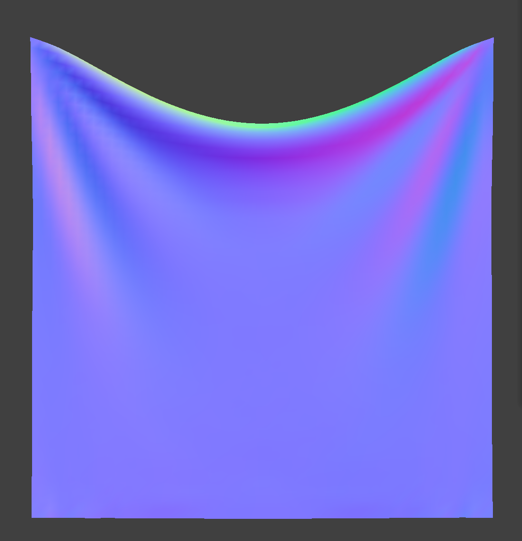
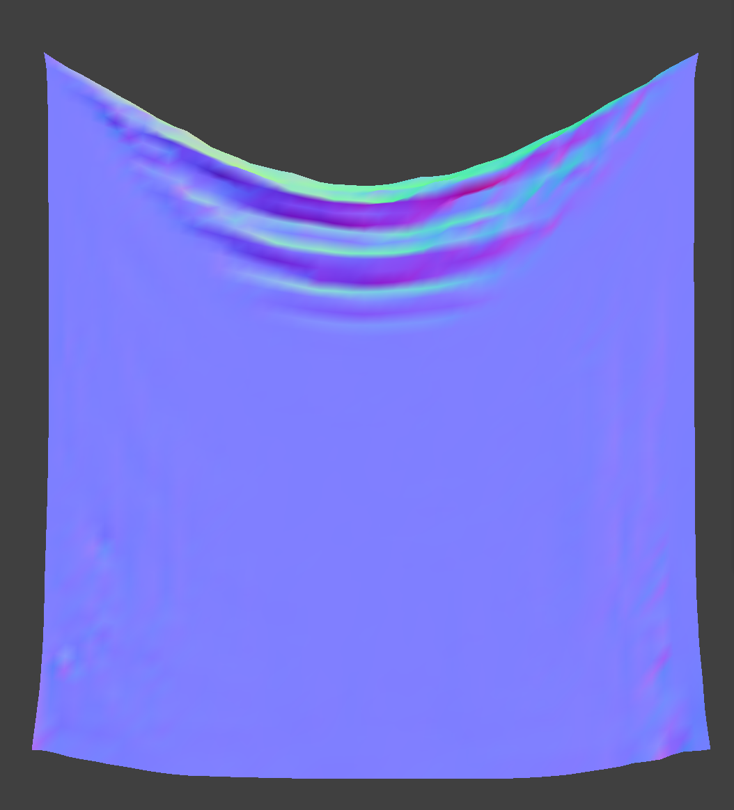
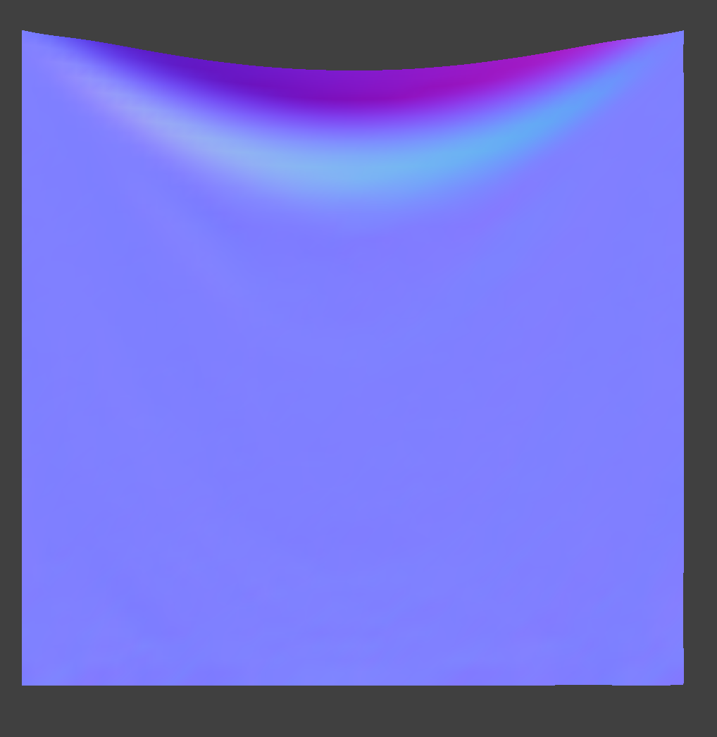
Changing the density affects how much the cloth is pulled downwards by gravity. A lower density means that the cloth will not be heavily affected by gravity, whereas a higher density means that the cloth will be pulled down a lot more. For example, we can see that the cloth produced with a density of 100 has a more noticeable dip towards the top in comparison to the default, whereas the cloth produced with a density of 1 has almost no dip, indicating that gravity is barely pulling it down.

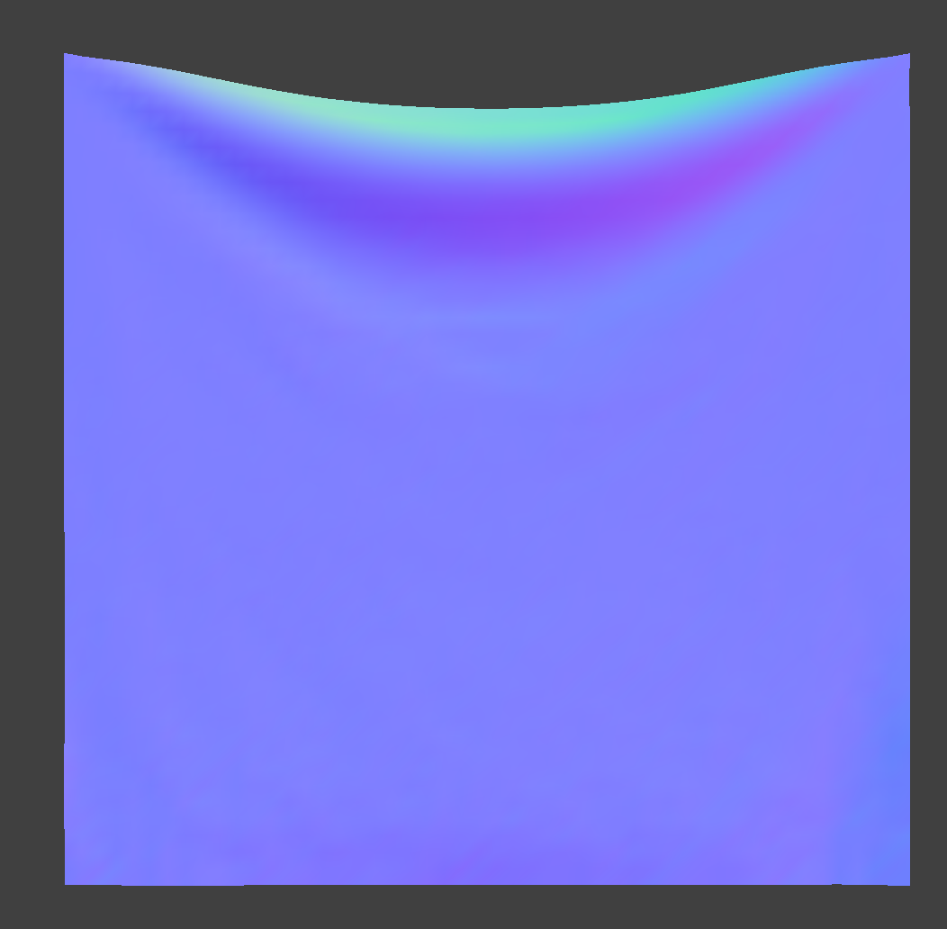
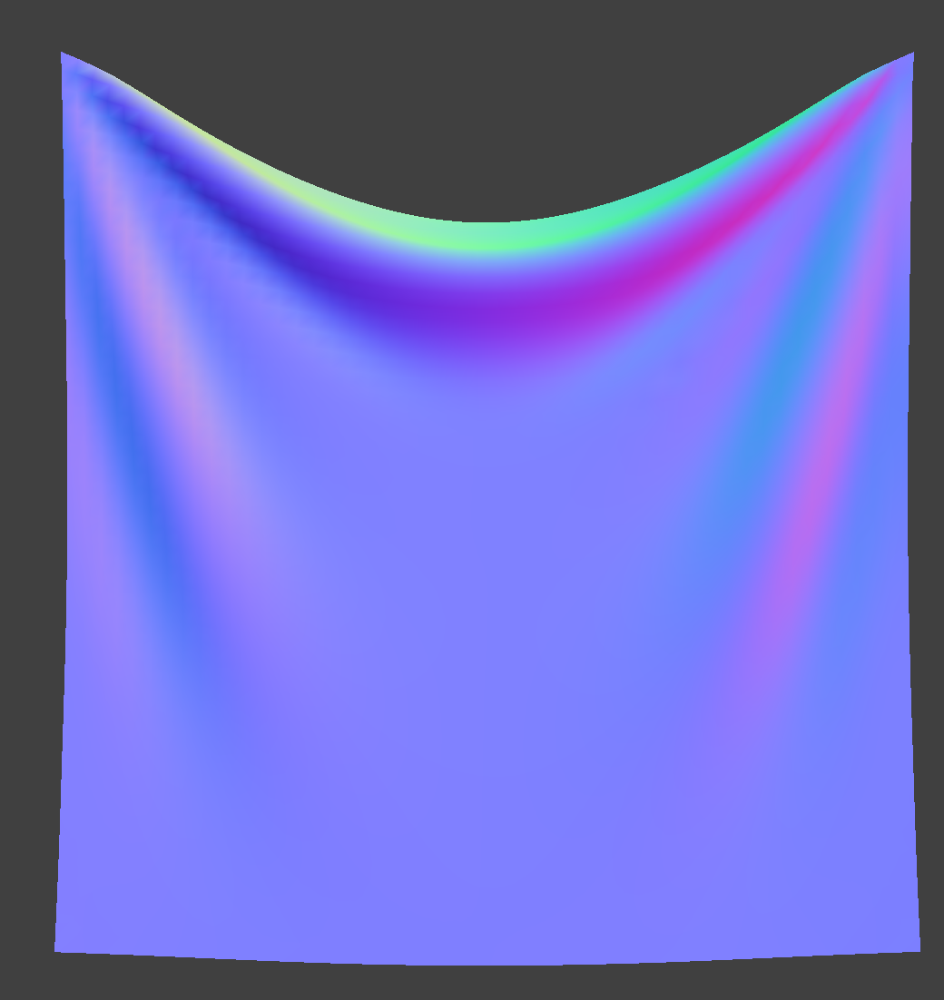
Changing the damping factor is related to how quickly a spring loses its energy and stops oscillating. When I set the damping value to 0.01, for example, the cloth swung back and forth dramatically and did not reach a stable resting state for quite a while. On the other hand, when I set the damping value to be much higher (0.8), the cloth had almost no oscillation at all, and reached its final resting state almost immediately.

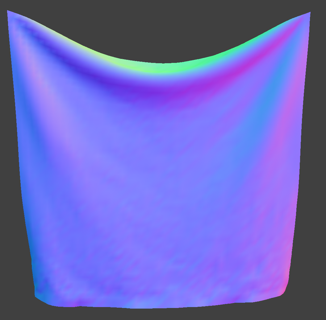
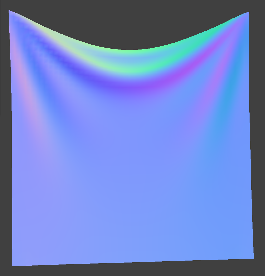
Section III: Handling collisions with other objects

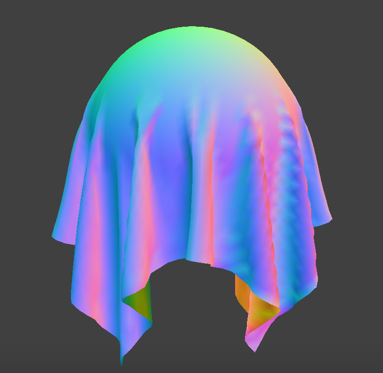
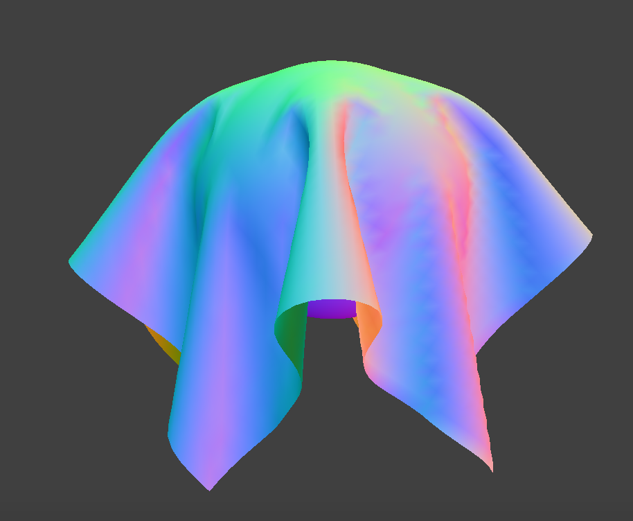
Handing collisions with spheres

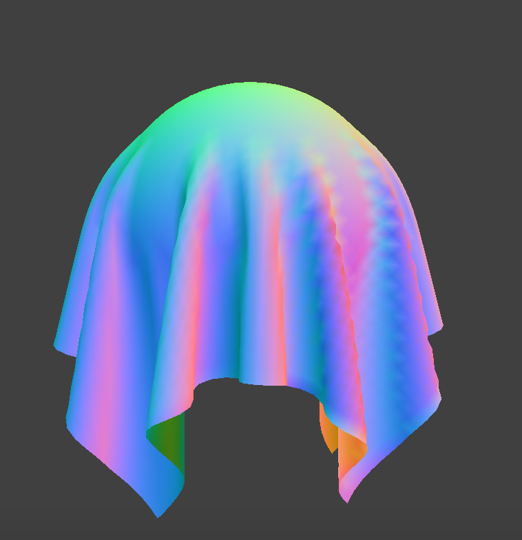
Compared to the default, having a lower ks value produced an image of a sphere where the cloth sagged a little more, implying a greater flexibility in the fabric. In contrast, when the ks value is super high, there are fewer wrinkles than that of the default because the cloth is much stiffer.

Handing collisions with planes

Below is a screenshot of a cloth resting peacefully on a plane.

Section IV: Handling self-collisions

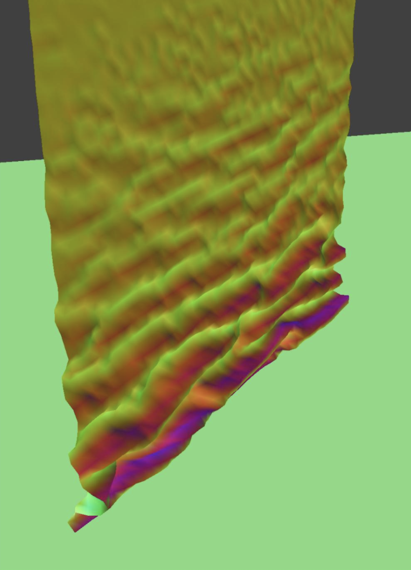
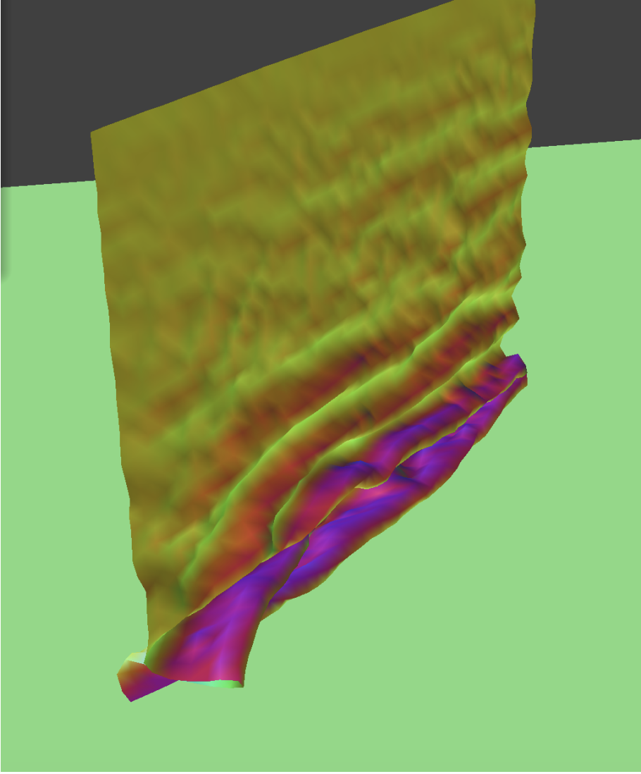
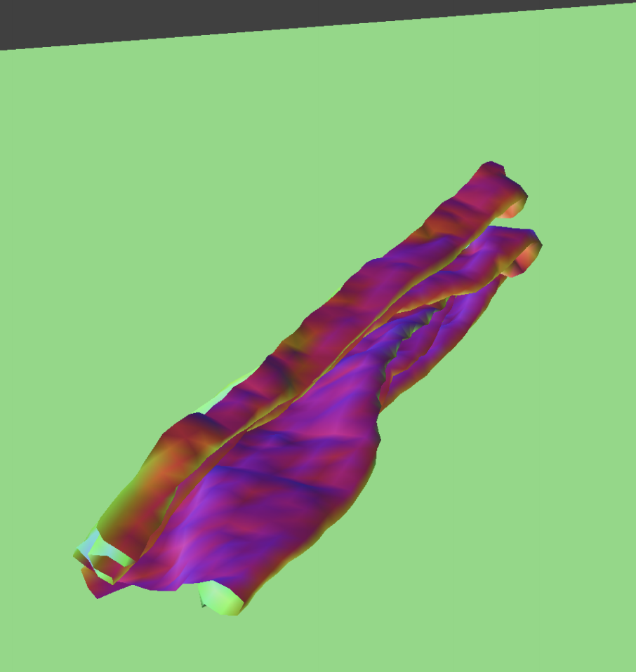
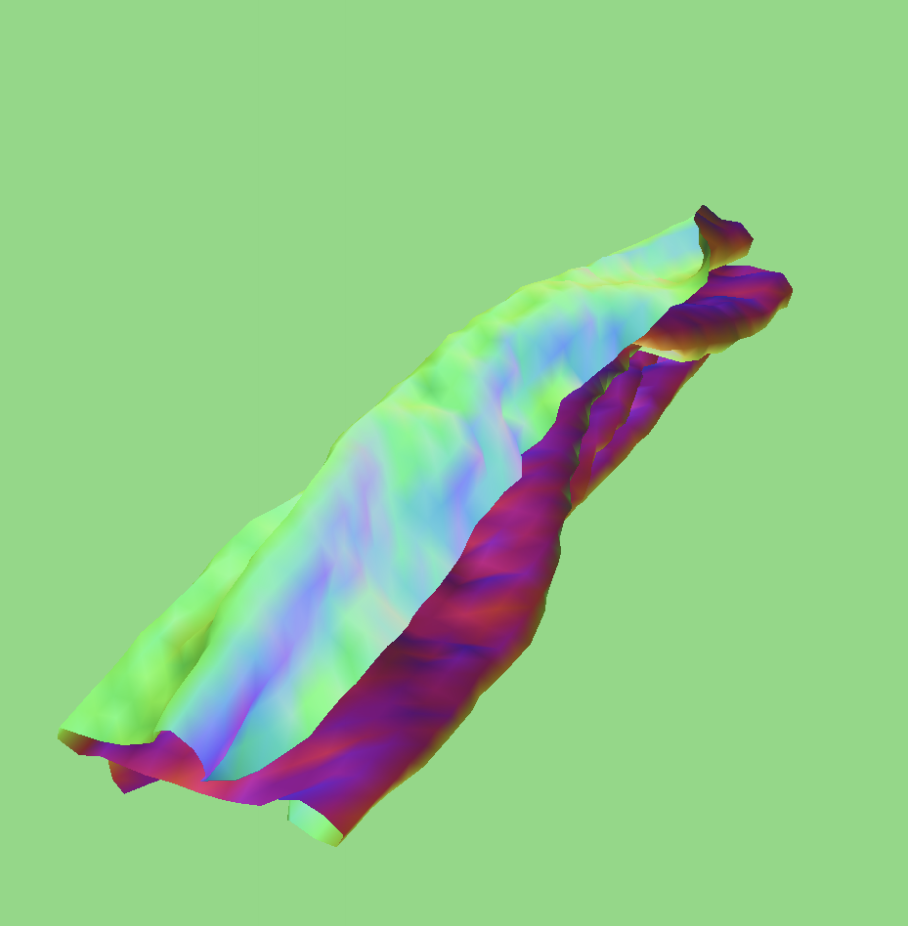
Self-Collision with default parameters

Self-Collision with Density = 1

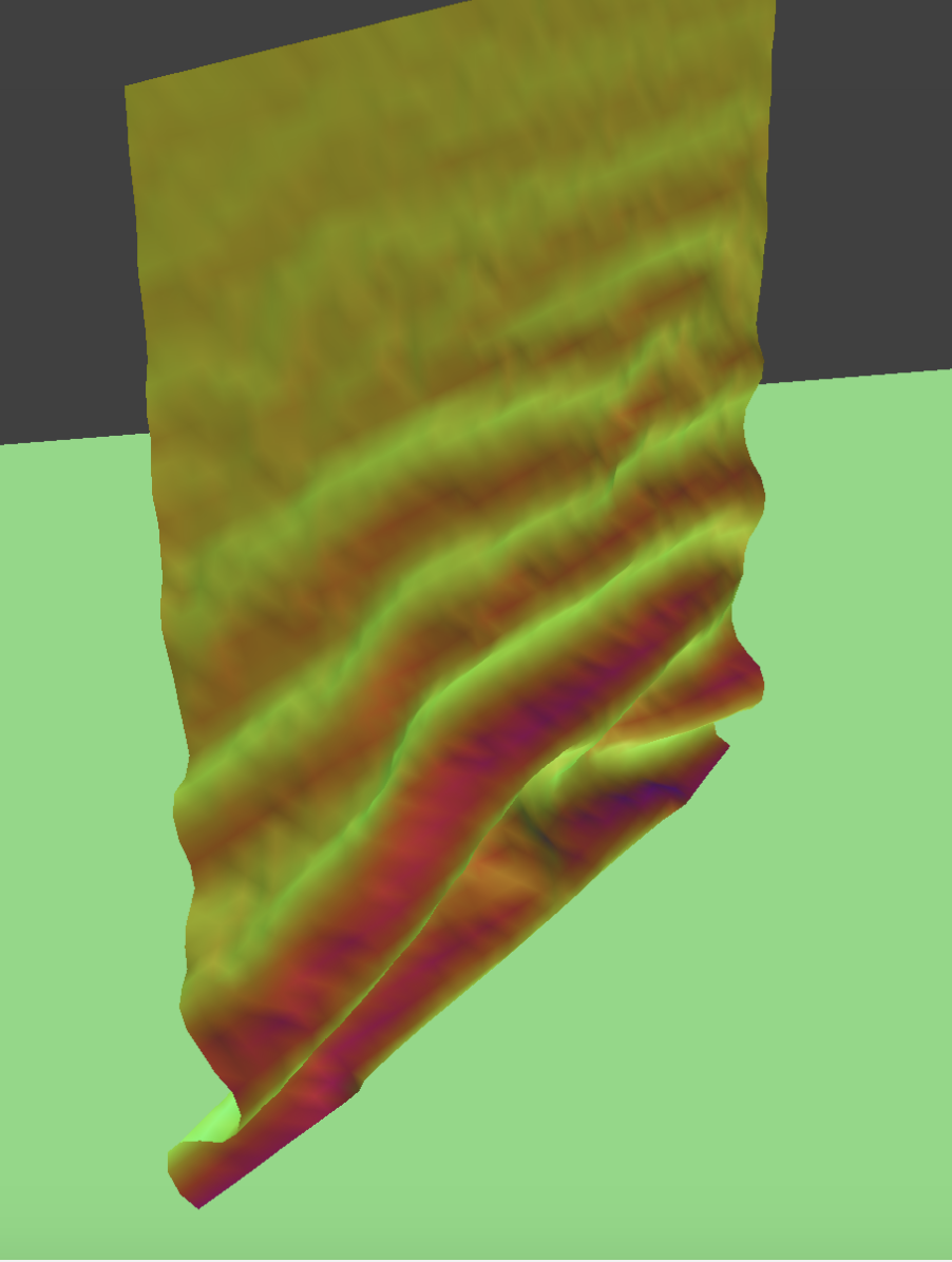
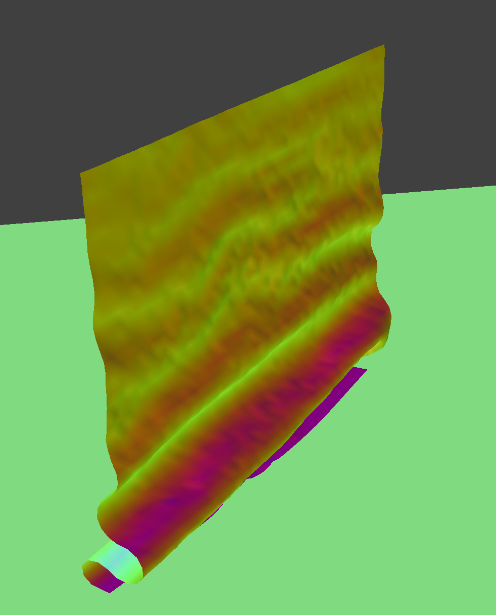
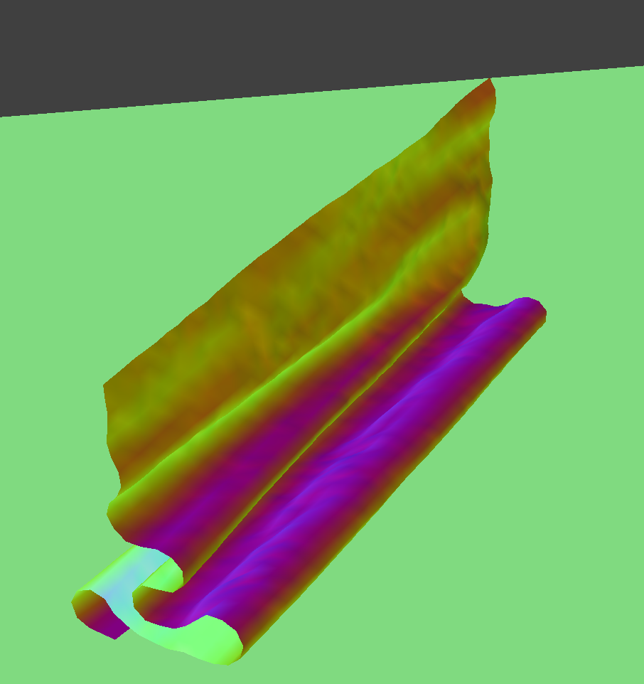
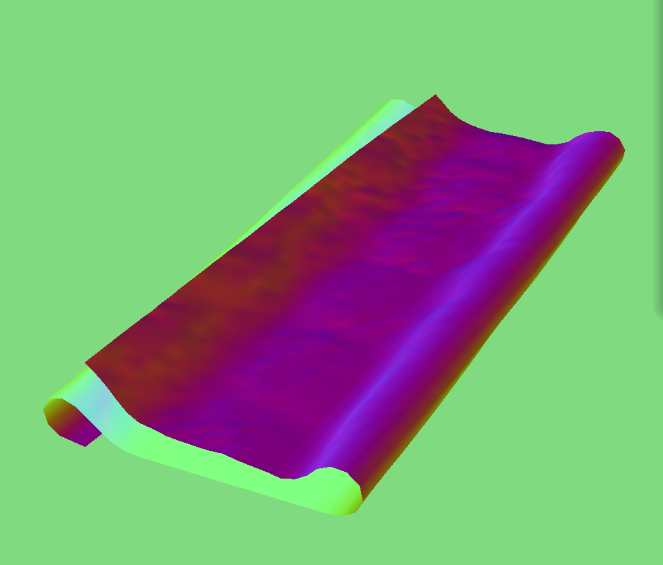
Self-Collision with Density = 50

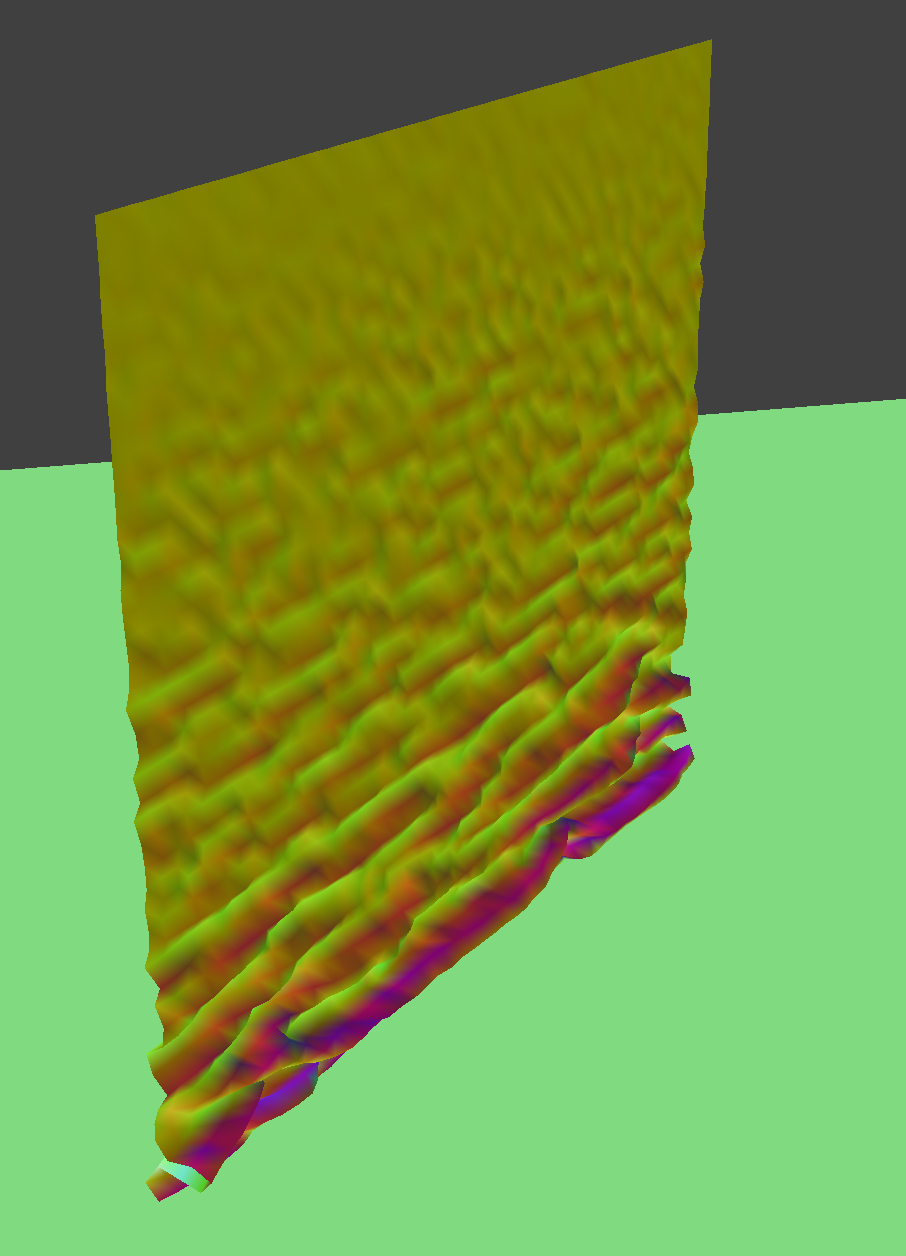
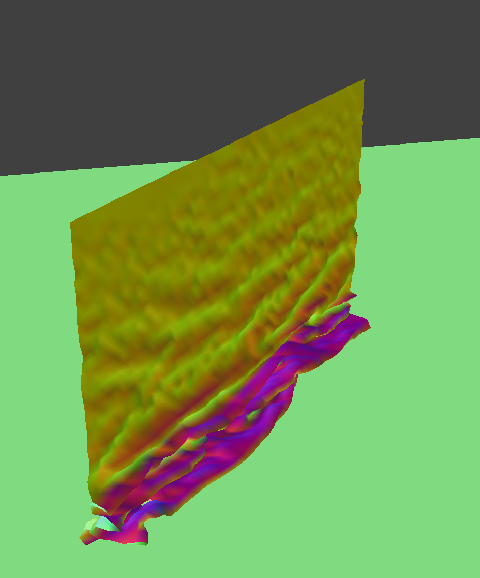
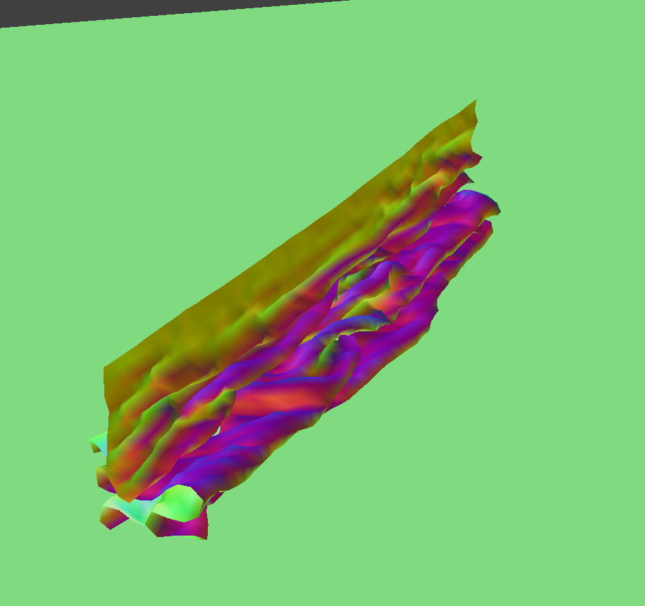
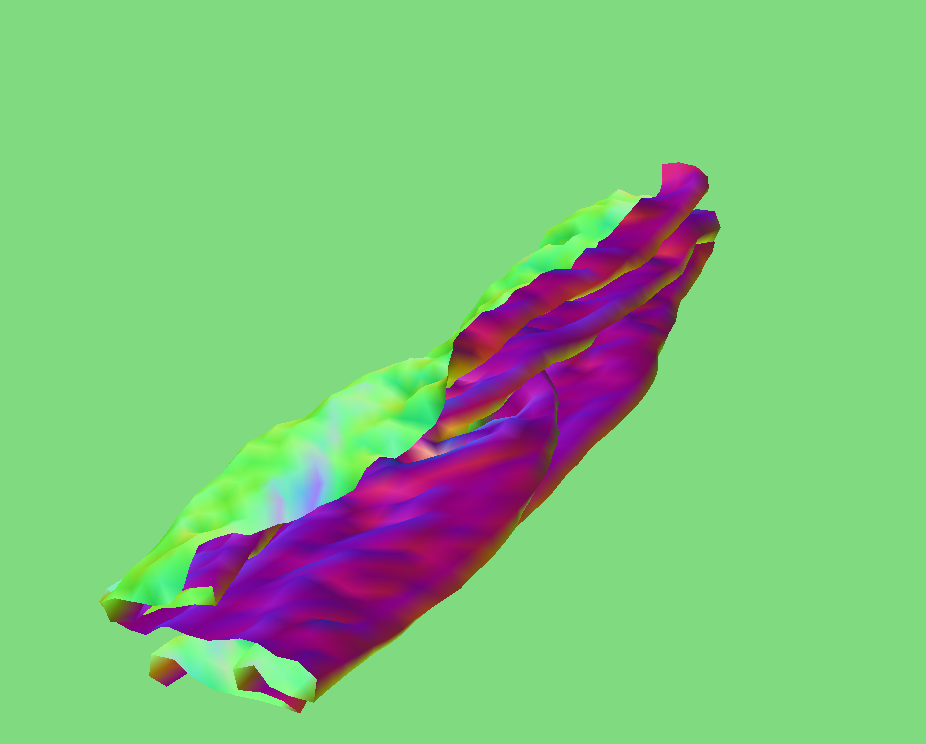
When I increase the density, the cloth folds over very wrinkled and flowy, whereas when I decrease the density, the cloth looks more rigid, and there are fewer creases.

Self-Collision with ks = 500

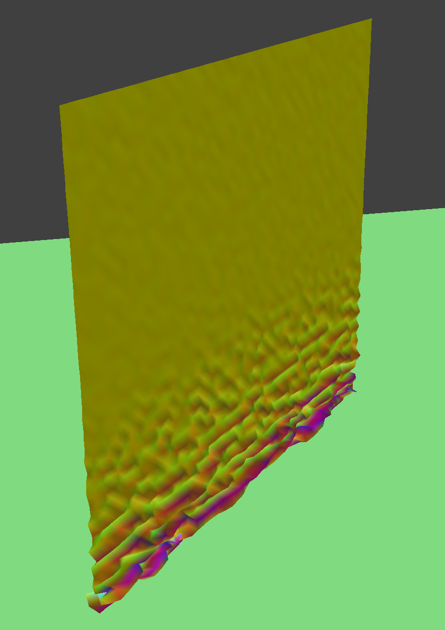
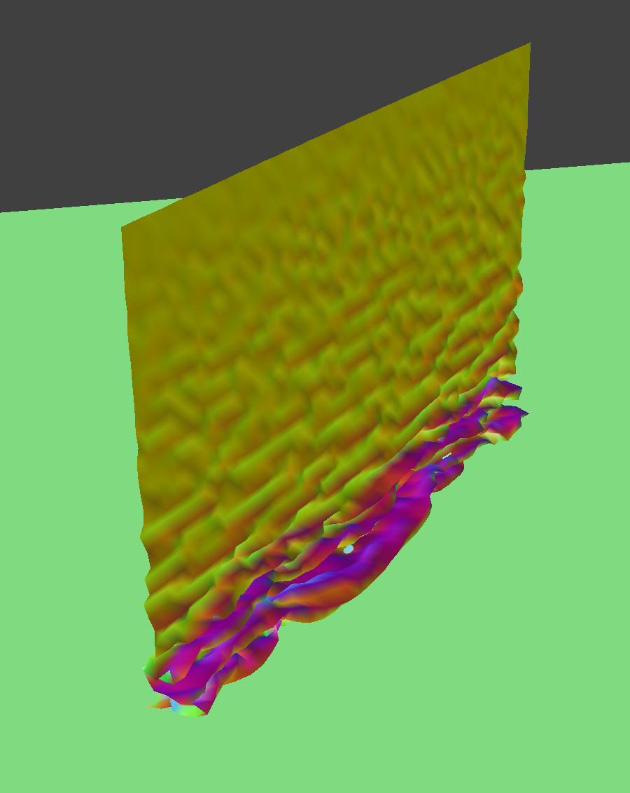
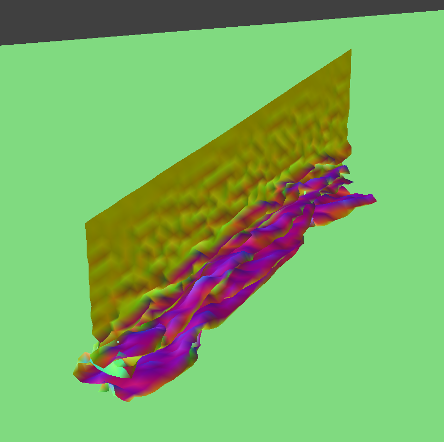
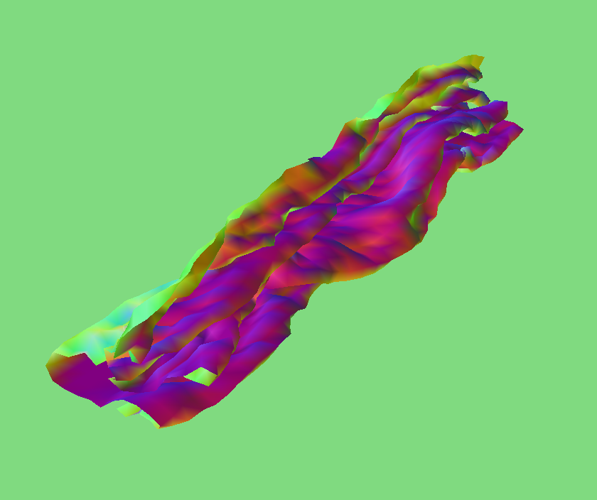
Self-Collision with ks = 50000

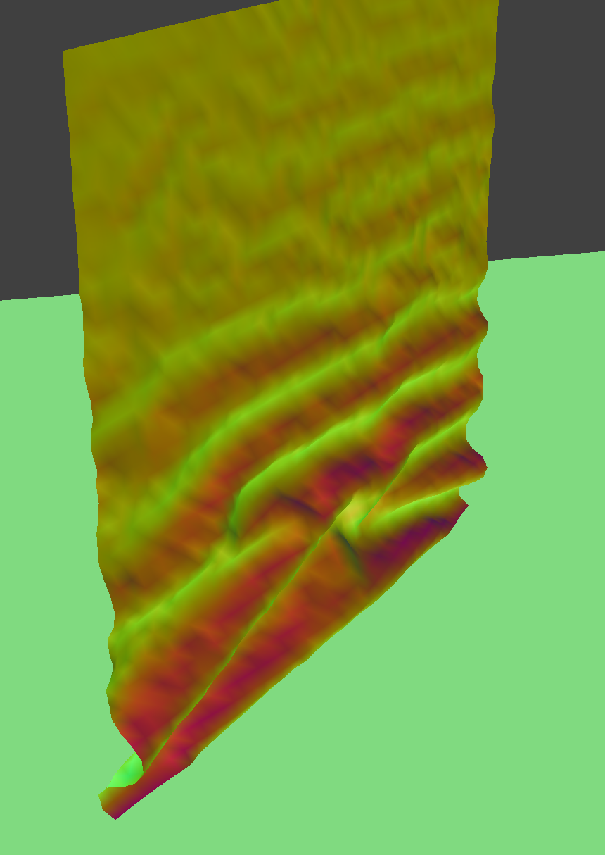
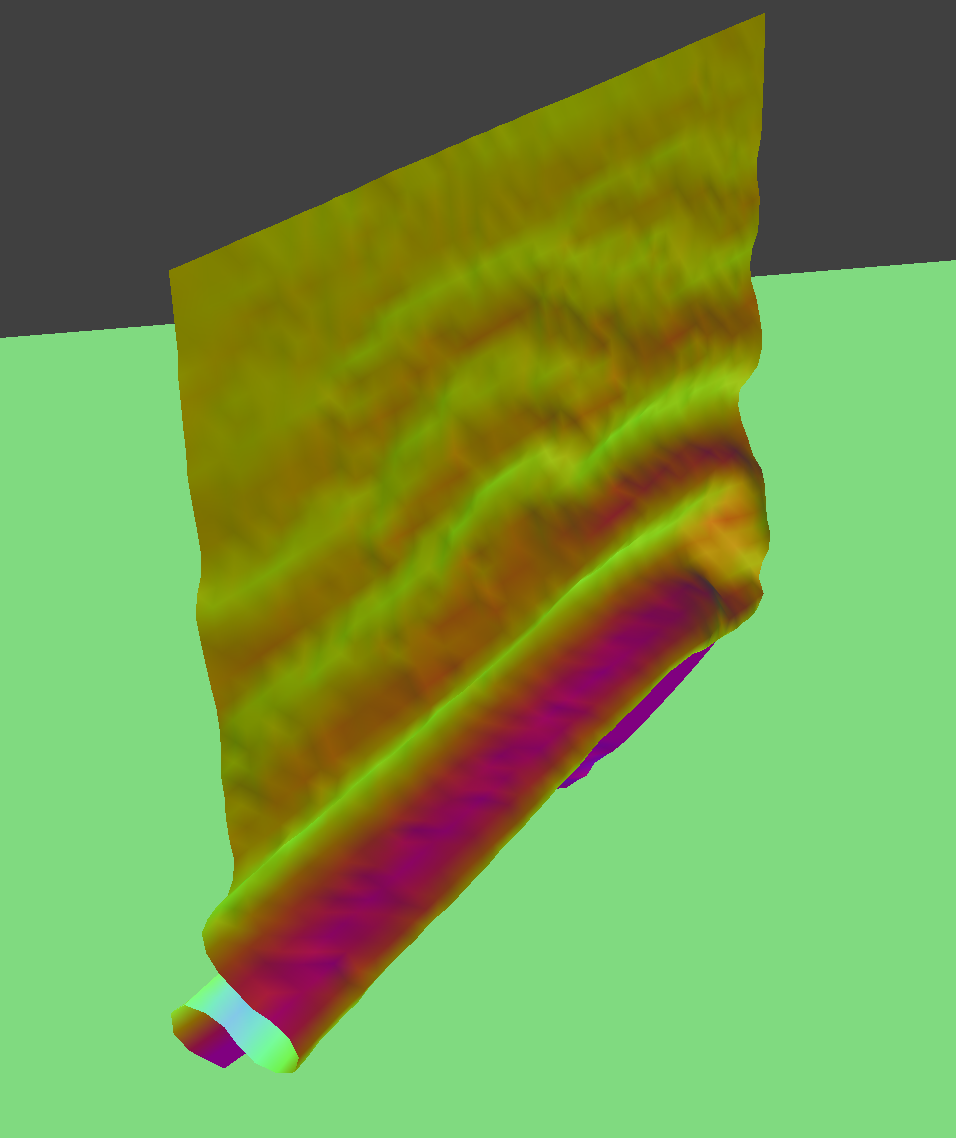
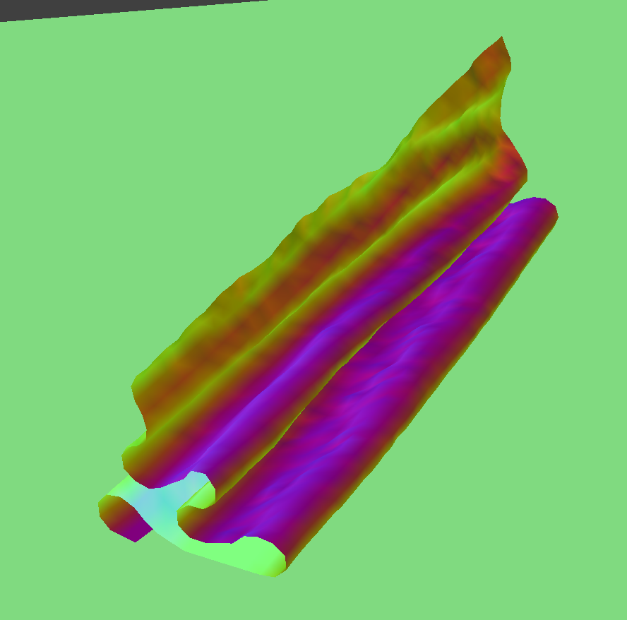
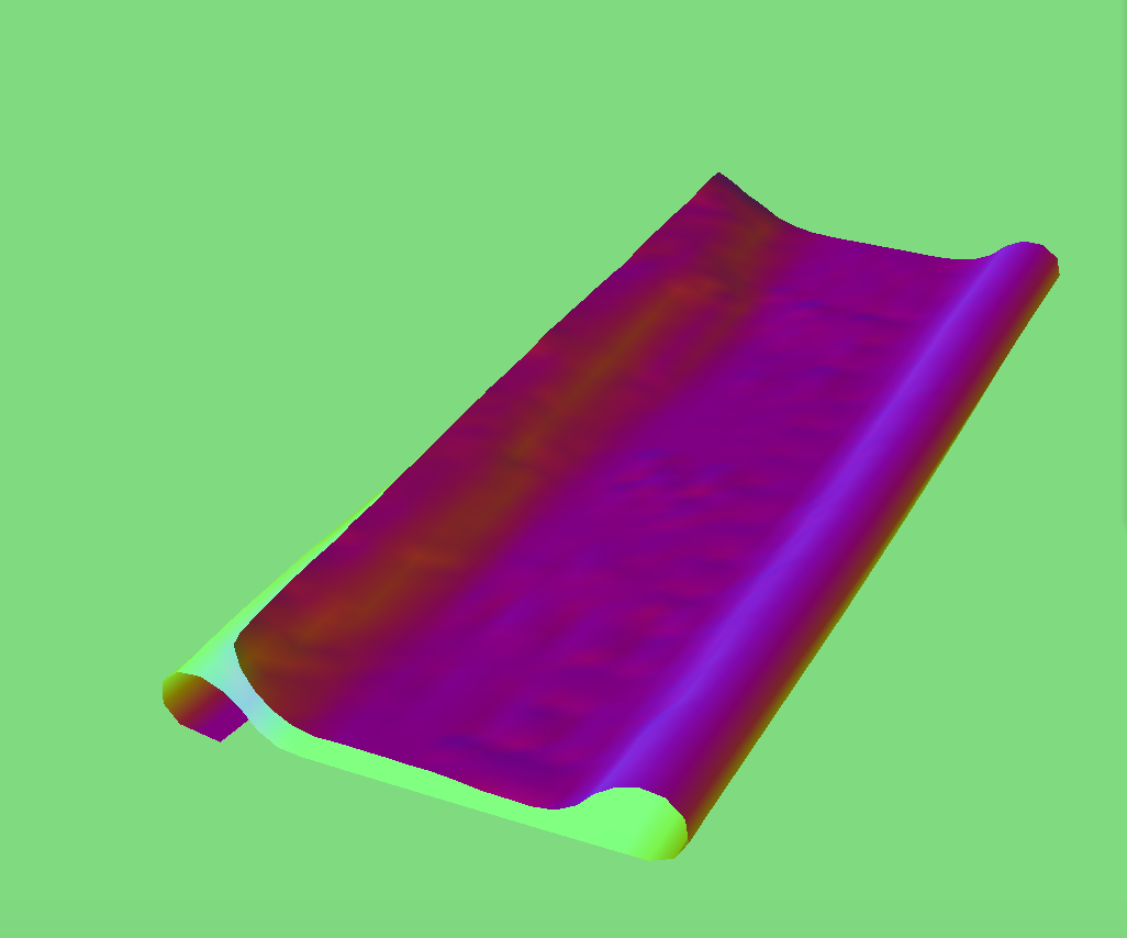
When I increase the ks value, the cloth looks stiffer for the reasons explained previously. When I decrease the ks value, the cloth looks like it has more give and looseness, implying that it is stretchier because of the low ks. Also, the cloth with a higher ks value takes much longer to reach its final resting state, matching what is expected because a high ks value increases the spring of the cloth.

Section V: Shaders

A shader program is one that runs in parallel on a GPU and outputs a 4D vector that contains information such as color and texture. Vertex shaders change vertex properties such as their position and normal vectors. Fragment shaders are used post-rasterization and compute the colors for pixels. Blinn Phong shading uses a combination of ambient and diffuse lighting and specular highlights to create a realistic shading model. It employs the formula below, where the first element accounts for ambient light, the second for diffuse, and the third for the specular highlights.

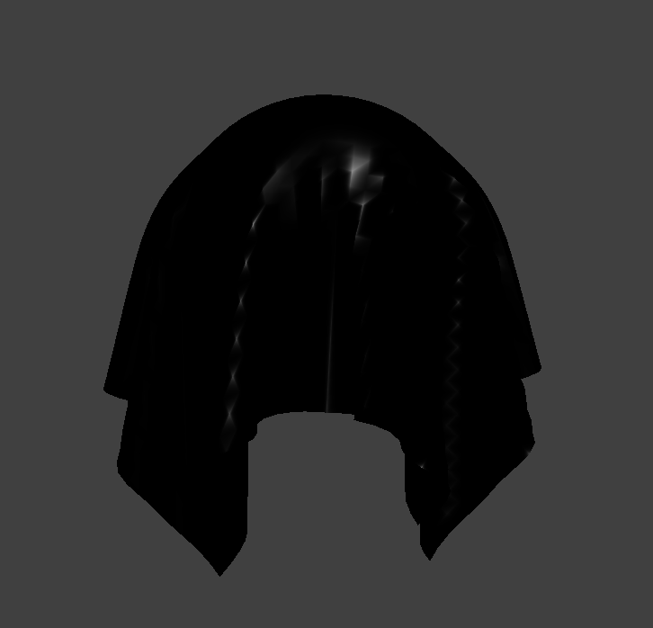
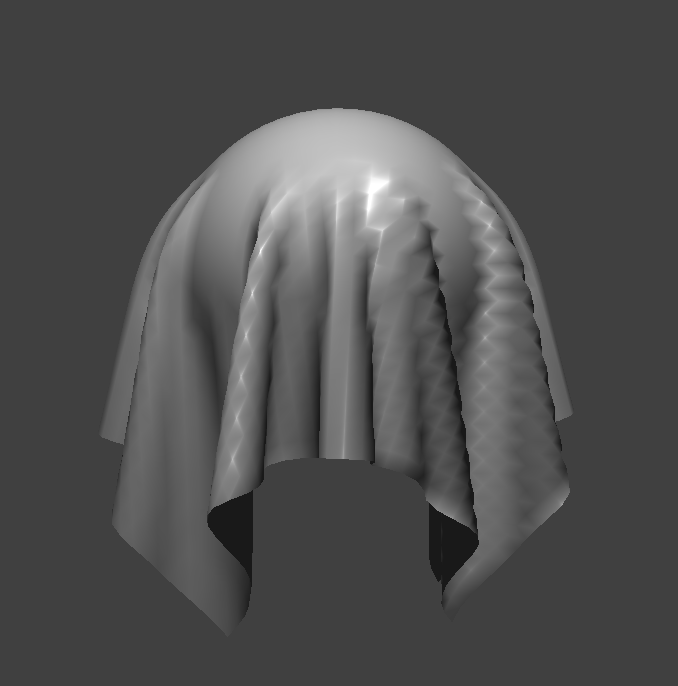
Below are screenshots of my Blinn-Phong shader outputting each of the components by themselves, and one using the entire Blinn-Phong model

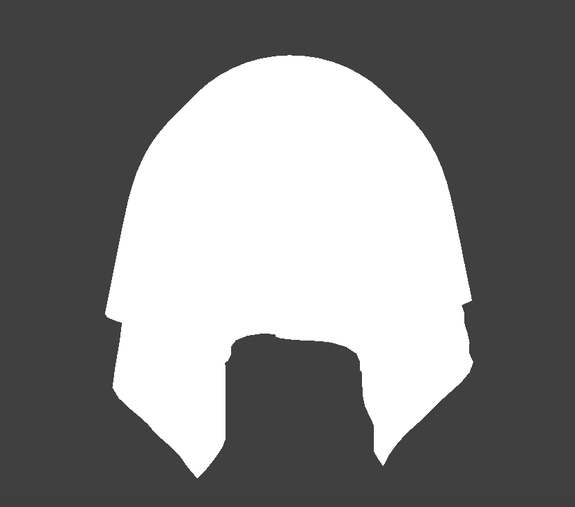
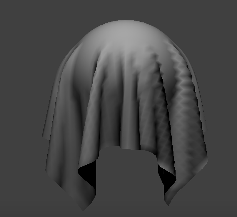
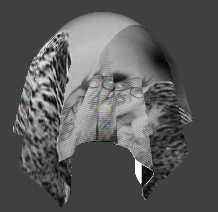
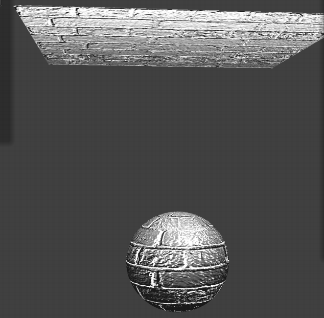
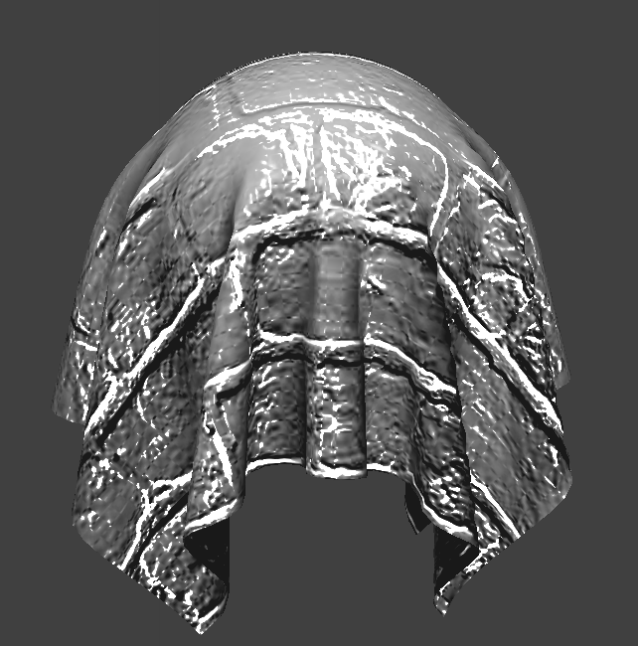
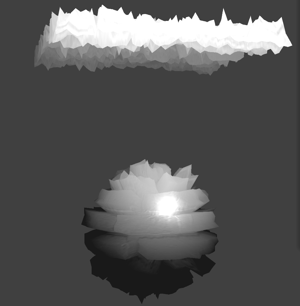
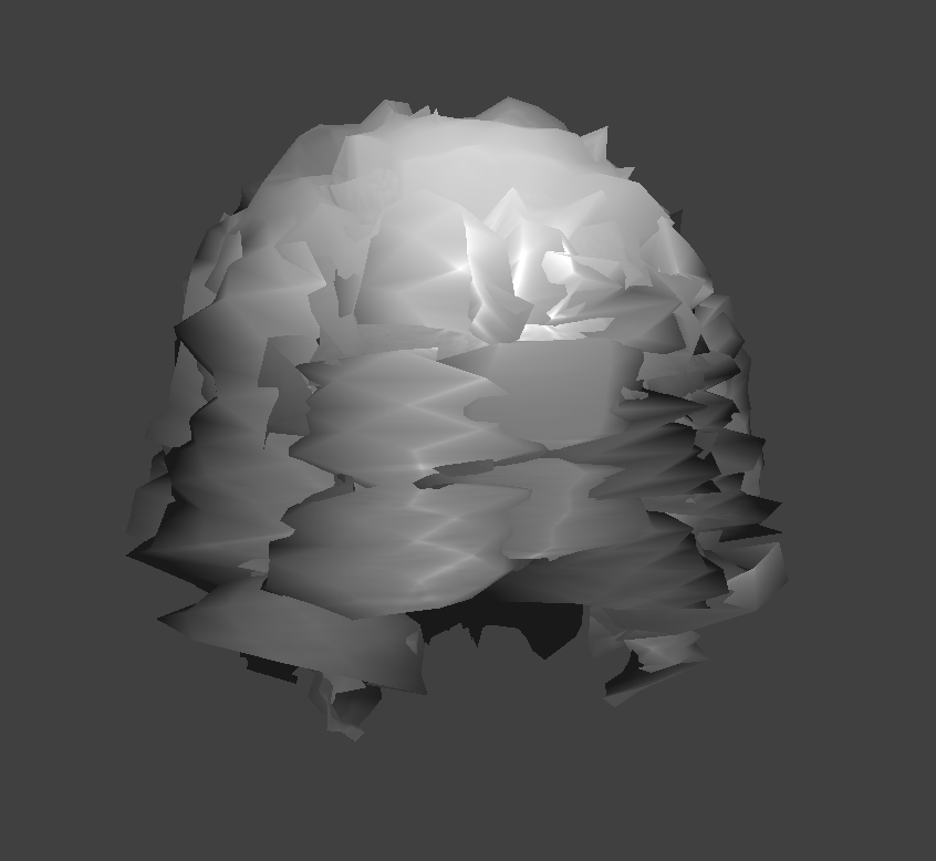
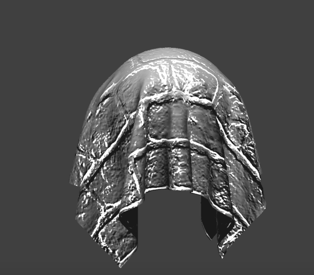
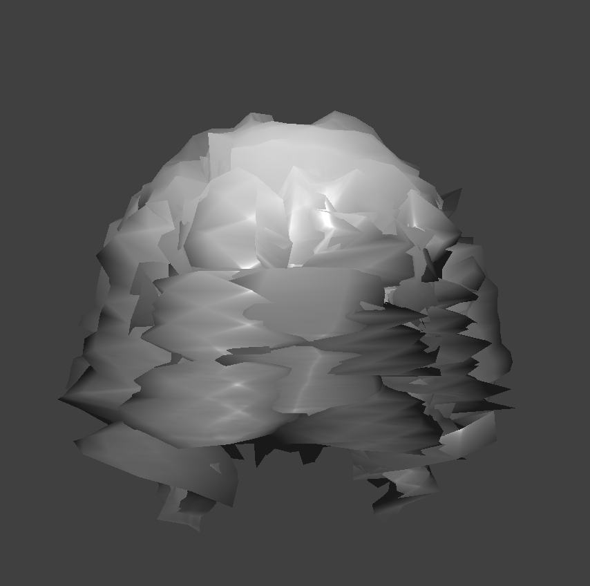
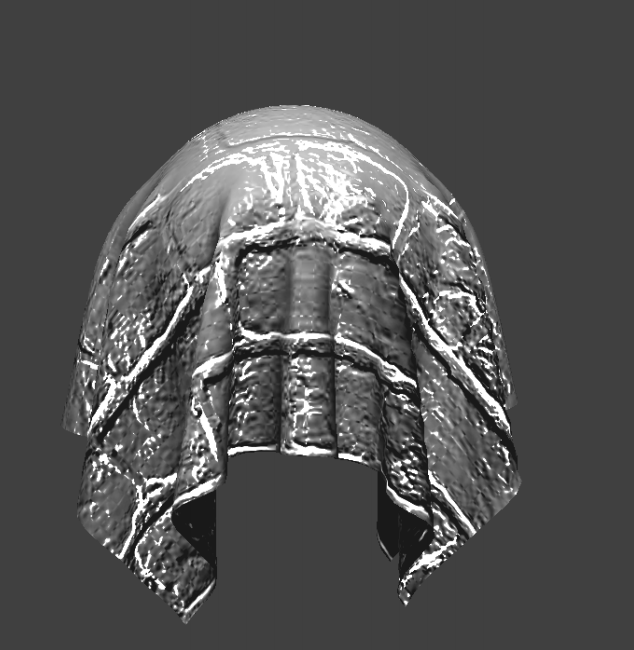
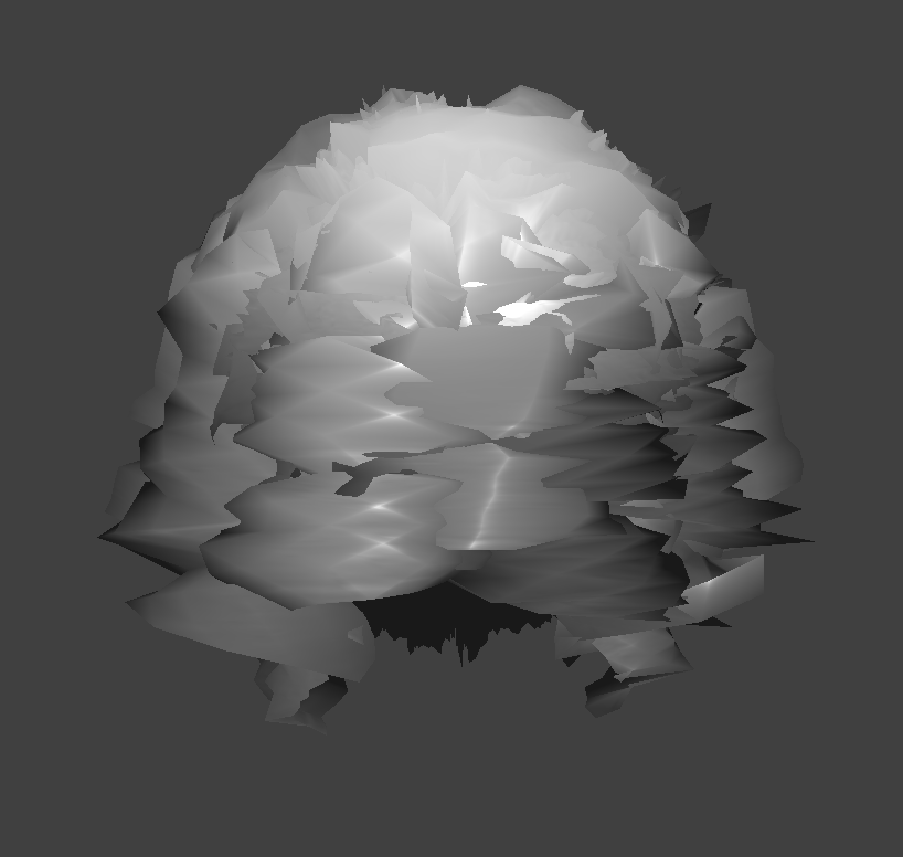
For the bump maps, I used a height of 10 and for the displacement maps, I used a height of 0.2. To implement bump mapping, I used the normals of the texture map to shade the surface changing the fragment shader, whereas for displacement mapping, I actually changed the surface itself through use of both the fragment and the vertex shader.

The following screenshots show how the two shaders react to the sphere by changing the sphere mesh's coarseness.